River Invertebrate Classification Tool (RICT) Functional Specification

1 Introduction

1.1 Purpose of the document

The purpose of this document is to define the business, functional and non-functional capabilities of RICT to support the design and implementation of RICT software tool.

The details will be sufficient to enable the software tool to be designed and built without having to continually refer queries to business representatives.

Further, it will be of sufficient detail to provide supporting documented information for any future RICT development.

1.2 Background

The UK Regulatory Agencies have a requirement to classify ecological quality in rivers using data from invertebrate samples. The RIVPACS (River InVertebrate Prediction and Classification System) model and software tool, which was developed on behalf of the agencies by the Freshwater Biological Association (FBA) and subsequently by the Centre for Ecology and Hydrology (CEH), was originally used for this purpose. It incorporates a set of summarised reference data from sites assumed to be the best available of their type.

The EU Water Framework Directive (WFD) introduced in 2000, included modifications to the regulatory requirements in relation to classification and therefore the RIVPACS software processing tool had to be amended.

The original RIVPACS software tool was written in FORTRAN and had been developed in stages over a number of years. As a result, it was not written in a modern programming language and did not have flexibility to allow changes without significant cost. Therefore, a new tool was developed that allowed future changes to be made with minimal cost in many cases (e.g. the addition of a new index). This was the River Invertebrate Classification Tool (RICT) version 1 which went live in 2007. This version of RICT was a web-served application which was accessed via a website hosted by SEPA. The SEPA website also hosted copies of the manual, guidance and background documents.

RICT has had some updates since 2007, including the addition of ‘split season’ classification to enable WHPT (Walley, Hawkes, Paisley and Trigg) calculations using seasonal average EQRs (Ecological Quality Ratio). RICT was managed and hosted by Scottish Environment Protection Agency (SEPA) but is also used by Environment Agency (EA), Natural Resources Wales (NRW) and Northern Ireland Environment Agency (NIEA) as part of their regulatory and statutory requirements as well as public users such as academic institutions.

However, a number of issues were identified with this version of RICT which can be found in the outline business case produced by the scoping project. These include improving the performance, support arrangements and resilience as well as adding the new RIVPACS model (RIVPACS version IV) to the RICT tool, resolving critical bugs and other additional functionality. The full list of Critical success factors can be found in Annex C.

A shortlist of options to resolve the issues was discussed which resulted in the recommendation that RICT should adopt a Platform as a Service arrangement and run a modified application.

A new cloud-based open source version of RICT was developed which incorporated the current RIVPACS IV model and WFD status classification and uses the same basic algorithms to provide the same final results (other than correction of errors). Code and data tables for the new version will be more accessible to developers who wish to further develop RICT. This new version of RICT is called RICT version 2 (RICT2).

The platform chosen for RICT2 was Microsoft Azure Machine Learning (ML) Studio with open source R programming language. Due to Azure closing down this service, the platform moved to a ‘Shiny’ web server hosted by Posit. This version is called RICT version 3 (RICT3). The code was moved to an R package on Github.

Advanced users can create their version of R code or run the R package locally on their machines.

The RICT web app and latest documentation including the technical specification and user guide via RICT web app.

2 Functional Overview

RICT is an application that implements the RIVPACS IV predictive model. The primary requirement of the tool is to allocate WFD (Water Framework Directive) compliant classifications to rivers with regard to the quality of the river invertebrate community.

The classifications are calculated and described as H() = high, G = good, M = moderate, P = poor or B = bad. This is achieved by comparing sample data from a river site against sample data previously taken from river sites considered to be the best available of their type.

The primary functions of the RICT tool are:

Predict - Predict the value of various biotic indices and the presence and abundance of invertebrate species, genera or families that you would expect at any place on any stream or river in the UK if it was not environmentally disturbed.
Classify - Determine the Water Framework Directive (WFD) quality status class and statistical information about its confidence.
Compare - Compare the statistical significance of differences between classifications.

It is to be capable of doing this for one or more sites at a time, with the results provided in an output file for subsequent processing by the relevant user.

The diagram below shows a diagrammatical representation of the main functionality of the RICT tool with numbered links to more detailed information.

3 Supporting files

RICT uses the RIVPACS reference data which contain sites that are considered to be the best available of their type. The latest version of the complete RIVPACS reference database for RICT can be downloaded from the RICT Website:

https://fba.org.uk/FBA/Public/Discover-and-Learn/Projects/RIVPACS-Reference-Sites-and-Reports.aspx

Within RICT, the RIVPACS reference data is not used at site level but is used at the End Group level, where an End Group contains combined data for sites considered to be of a similar biological composition. End Groups are grouped up to End Group Sets (e.g. New GB – 43 Group level).

As well as this data table, RICT needs other data which will be held and used as internal data tables and R software code functions.

All the following files can be found within the rict package on github.

The rict code is automatically tested and compiled/built on every update to the master branch on Github. This process is carried out by the Github actions website, which monitors repo for any changes and re-builds and tests the code on a Windows, Mac and Linux machine in the cloud. It then automatically deploys updates to the web app and/or documentation.

3.1 Prediction

3.1.1 Support Tables:

These files can be found in the inst/extdat folder within the rict package.

Model 1 specific:

Files used in calculate discriminant function scores section:

df-coeff-gb-685.DAT – GB
df-coeff-iom.DAT - Isle of Man
DFCOEFF_NI.DAT - NI

Files used in calculating Mahanalobis distance section:

DFMEAN_NI_RALPH.DAT - NI
df-mean-gb-685.DAT - GB
df-mean-iom.DAT - IoM

Files used for calculating proportion during prediction: * endGrp-AssessScoresNI.csv - NI * end-grp-assess-scores.csv - GB * end-grp-assess-scores-iom.csv - IoM

Model 44 specific:

discrimintant-function-coefficient-model-44.csv - used for discriminant score.
discrimantinant-function-model-44.csv file used for calculating Mahanalobis distance.

For both models:

air-temp-grid.csv – contains previously derived Environmental data values for the Mean Air Temperature (TEMPM) and Temperature range (TEMPR) for points in the centres of 5km interval grid squares. Values are used after converting the supplied NGR (or BNR) to latitude and longitude to identify the relevant values required. Not used for Isle of Man.
TAXA_AB_APR_PRAB.csv - containing abundance and probability of abundance category for each taxon used in predicting taxa.
x-103-end-group-means-formatted-jdb-17-dec-2019.csv – combined data for sites considered to be of a similar biological composition the End Group table used in RICT is called

3.1.2 Prediction Functions:

Found in the /R package directory there are two main R functions files for predictions:

rict-predict.R - main function called to run prediction
rict-validate.R - lower level function to validate input data helper-functions.R - support functions to carry out the Environmental Variables validation

Prediction support functions are found:

prediction-functions.R
calc_temperatures.R

3.2 Classification

Note, no classification is carried out on the 80 indices – carried out for Prediction only!

3.2.0.1 Classification Functions:

classification-functions.R - A large number of R code functions used in the classification section.

3.2.0.2 Classification support files:

adjustParams_ntaxa_aspt.csv - reference adjustment values.
adjustParams_ntaxa_aspt.csv containing reference adjustment values which are used as described in Adjust Expected Values section.
endGrp-AssessScoresNI.csv & end-grp-assess-scores.csv & end-grp-assess-scores-iom.csv used for Adjust Expected Values section.

All source code and support files can be downloaded into R environment for example Rstudio from Github for users who wish to amend and create their own versions.

4 RICT

4.1 Default values

The list below describes the default values used:

Number of Monte-Carlo simulations – 10,000
Index sets – all 80 indices
Season type – Spring, Autumn, Spring/Autumn Combined, Summer
Classification boundary limits – Coded as per WFD compliant values found in the classification support files (user would need to amend the function in this file to alter values for their own version)
Bias - Bias values can be provided in the input file by the user and will be used if provided. However, if no data values for Bias or “-9” has been entered in the input file, then the hard-coded default value of 1.68 (GB + IoM) or 0 (NI) will be used.

Note that 1.62 value was used for Bias as this was the default input value in the previous version of RICT as used in SEPA for BMWP NTAXA. However, the EA uses a value of 1.68 as the Bias value for WHPT which was based on an audit of the analytical quality of Environment Agency laboratories. The Bias value for WHPT should be greater than the value for BMWP for the same level of analytical quality, because WHPT uses more taxa than BMWP. Plus WHPT taxa also includes additional Diptera families which are less easy to identify.

4.2 Future Developments

A multi-site classification will be added to enable water bodies to be classified from more than one site. The GIS data location checker and delivery system and multi-site classification are currently in development and we hope to release them in a couple of months.

Additional standard default to calculate the output for more specific Index sets (e.g. for hydro-ecological evaluation) may be added later, if the need arises.

Future RICT release may allow a user to run predictions and classifications against previous classifications and RIVPACS models to allow historical data to be analysed in a consistent way with current monitoring data. That may include BMWP (Biological Monitoring Working Party) classification based on RIVPACS IV (used before 2015) or RIVPACS III+ (used 1990-1009), or using WHPT based on BMWP taxa including BMWP composite taxa.

We may correct or improve features, if we need to do that, we will run them through testing and add to this document and user guides, as appropriate.

5 Acceptance and validation of input data

In order to be able to predict and classify, the tool requires input data in one csv file which includes:

Site Identifier
Values for a number of Environmental Variables (e.g. NGR, slope, discharge, etc.)
Values for a number of Observed Tool Indices (e.g. ASPT, NTAXA, etc.) (only required for classification)

An excel spreadsheet template will be provided for the user to enter input data into the relevant column headings. Validation rules will be applied to the data that has been input for each column to help the user meet the validation requirements detailed below.

The input data spreadsheet template can be found in Annex A of this document. Once completed, this spreadsheet will need to be saved as a csv format and uploaded by the user.

5.1 Environmental Variable Values and Validation

Environmental Variables (EV) are needed to enable the prediction process to calculate the probability of end group membership. The values of some Environmental Variables are provided and input by the user. The values of other Environmental Variables have to be derived using the values of one or more provided Environmental Variables and then converted. The complete set of input and derived Environmental Variables used by RICT are called Predictive Environmental Variables (PEVs).

The tables below refers to the Environmental Variable data required and the data field validation for the RIVPACS IV Great Britain and Northern Ireland Model M1 and additionally the model M44. The M1 model requires input of 13 PEVs for Great Britain and 11 PEVs for Northern Ireland. M44 model required 17 PEVs.

Input file screening will be carried out using the rules described in the tables below when a user enters data into the input file spreadsheet. This will be done by the conditional formatting tool within the MS Excel ribbon to check and highlight to the user where data does not meet validation requirements. It will highlight failures in red and warnings in orange. However, it will not stop the user from supplying that data to RICT for processing. When RICT processes the data, the appropriate Fail and Warn errors will be generated as described below.

Validation has also been coded into RICT for validation of the value ranges, i.e. “all”, “gb” and “ni”.

Note that at least one set of the following data will be required for each site but there may be up to three sets of data where the ‘raw’ data is being provided for up to three years for multi-year classification.

5.1.0.1 Input variables

All input variables as well as their validation rules are listed in the validation-rules.csv file within the package. The tables below are generated from this file.

5.1.0.2 Model 1 User input file

Required values (including using physical predictors) :

	Variable	Units	Description	Type	Optional
1	SITE		Site	character	FALSE
2	WATERBODY		Waterbody	character	TRUE
3	YEAR		Year	integer	FALSE
4	NGR		National Grid Reference	character	FALSE
5	EASTING	m	Easting	character	FALSE
6	NORTHING	m	Northing	character	FALSE
7	ALTITUDE	m	Altitude	numeric	FALSE
9	SLOPE	m/km	Slope at site	numeric	FALSE
11	DISCHARGE		Discharge Category	numeric	TRUE
13	VELOCITY	m/s	Velocity	numeric	TRUE
15	DIST_FROM_SOURCE	km	Distance from Source	numeric	FALSE
17	MEAN_WIDTH	m	Stream Width	numeric	FALSE
19	MEAN_DEPTH	cm	Stream Depth	numeric	FALSE
21	BOULDER_COBBLES	%	Boulder Cobble Percentage	numeric	FALSE
22	PEBBLES_GRAVEL	%	Pebbles Gravel Percentage	numeric	FALSE
23	SAND	%	Sand Percentage	numeric	FALSE
24	SILT_CLAY	%	Silt Clay Percentage	numeric	FALSE
25	HARDNESS	%	Hardness	numeric	TRUE
26	CALCIUM		Calcium Concentration	numeric	TRUE
27	CONDUCTIVITY		Electrical Conductivity	numeric	TRUE
28	ALKALINITY	mg/L	Alkalinity as CaCO3	numeric	FALSE

5.1.0.3 Model 44 Input files (using GIS predictors)

Required values:

	Variable	Units	Description	Type	Optional
1	SITE		Site	character	FALSE
2	WATERBODY		Waterbody	character	TRUE
3	YEAR		Year	integer	FALSE
4	ALKALINITY	mg/L	Alkalinity as CaCO3	numeric	FALSE
6	DISCH_CAT		Discharge Category	numeric	FALSE
7	PEAT	Proportion	Peat	numeric	FALSE
8	CHALK	Proportion	Chalk	numeric	FALSE
9	CLAY	Proportion	Clay	numeric	FALSE
10	HARDROCK	Proportion	Hardrock	numeric	FALSE
11	LIMESTONE	Proportion	Limestone	numeric	FALSE
12	LOG_AREA	Log (km2)	Log Area	numeric	FALSE
13	LOGALTBAR	m	Mean Altitude of Catchment	numeric	FALSE
14	ALTITUDE	m	Site Altitude	numeric	FALSE
15	D_F_SOURCE	m	Distance from Source	numeric	FALSE
16	SLOPE	m/km	Slope at site	numeric	FALSE
17	SX		Sampling Site X Coordinate (BNG)	numeric	FALSE
18	SY		Sampling Site Y Coordinate (BNG)	numeric	FALSE

5.1.0.4 Optional values

Columns containing optional values must still be present in input data file but all or some of their values may be missing (data type NA). However, they must comply with the following notes:

5.1.0.5 Model 1 Optional notes:

	Variable	Optional note
1	DISCHARGE	One of DISCHARGE or VELOCITY
3	VELOCITY	One of DISCHARGE or VELOCITY
5	HARDNESS	One of Alkalinity, Hardness, Conductivity or Calcium
6	CALCIUM	One of Alkalinity, Hardness, Conductivity or Calcium
7	CONDUCTIVITY	One of Alkalinity, Hardness, Conductivity or Calcium
8	ALKALINITY	One of Alkalinity, Hardness, Conductivity or Calcium

5.1.0.6 Model 44 Optional notes:

Variable	Optional note
ALKALINITY	One of Alkalinity, Hardness, Conductivity or Calcium

5.1.0.7 Validation

Warnings: Where the value of an environmental input variable exceeds a “Warn” limit, the prediction process will continue but warning message is created for that particular site.

Fails: Where the value of an environmental input variable exceeds a “Fail” limit, the prediction process will not proceed for that particular site and flags the transgression in a fail message.

5.1.0.8 Validation rules for Model 1

Variable	Area	Less than fail	Greater than fail	Less than warn	Greater than warn
SITE	all	0.00	NA	NA	NA
WATERBODY	all	0.00	NA	NA	NA
YEAR	all	0.00	NA	1990.0000000	NA
NGR	all	NA	NA	NA	NA
EASTING	all	NA	NA	NA	NA
NORTHING	all	NA	NA	NA	NA
LATITUDE	gb	49.95	60.86	49.9978431	60.8034893
LATITUDE	ni	54.02	55.38	54.0684100	55.1995835
LONGITUDE	gb	-7.67	1.76	-7.3651894	1.3560119
LONGITUDE	ni	-8.20	-5.43	-8.0916181	-5.7731300
ALTITUDE	gb	0.00	1345.00	0.0000000	590.0000000
ALTITUDE	ni	0.00	850.00	3.0000000	180.0000000
SLOPE	gb	0.00	NA	0.1000000	150.0000000
SLOPE	ni	0.00	NA	0.1000000	50.0000000
DISCHARGE	gb	1.00	10.00	NA	9.0000000
DISCHARGE	ni	1.00	10.00	NA	8.0000000
VELOCITY	gb	1.00	5.00	NA	NA
VELOCITY	ni	1.00	5.00	NA	NA
DIST_FROM_SOURCE	gb	0.00	NA	0.1000000	202.8000000
DIST_FROM_SOURCE	ni	0.00	NA	2.2000000	75.0000000
MEAN_WIDTH	gb	0.00	NA	0.4000000	116.7000000
MEAN_WIDTH	ni	0.00	NA	2.0000000	37.2000000
MEAN_DEPTH	gb	0.00	NA	1.7000000	300.0000000
MEAN_DEPTH	ni	0.00	NA	15.0000000	183.0000000
BOULDER_COBBLES	all	0.00	100.00	NA	NA
PEBBLES_GRAVEL	all	0.00	100.00	NA	NA
SAND	all	0.00	100.00	NA	NA
SILT_CLAY	all	0.00	100.00	NA	NA
MSUBST	gb	NA	NA	-7.7050000	8.0000000
MSUBST	ni	NA	NA	-7.7500000	6.6125000
HARDNESS	all	NA	NA	NA	NA
CALCIUM	all	NA	NA	NA	NA
CONDUCTIVITY	all	NA	NA	NA	NA
TEMPM	gb	0.10	NA	7.5000000	11.5000000
TEMPR	gb	0.10	NA	8.2100000	13.9000000
ALKALINITY	gb	0.00	NA	0.7000000	365.5000000
ALKALINITY	ni	0.00	NA	2.5000000	193.5000000
TOTSUB	all	97.00	103.00	NA	NA
DIST_FROM_SOURCE	iom	0.00	NA	0.1000000	13.1000000
ALTITUDE	iom	0.00	621.00	0.0000000	219.0000000
SLOPE	iom	0.00	NA	0.1000000	166.6700000
ALKALINITY	iom	0.00	NA	0.7000000	126.6000000

Model 1 Validation notes:

Variable	Validation notes
YEAR	Warn if samples collected prior to 1990 as unlikely to be collected using RIVPACS method
NGR	Must be less than 3 letters, can be upper or lower case
EASTING	Must be 5 digits; text not number, to retain leading zeros (input file screening). In R Code: If less than 5 digits add leading zeros
NORTHING	Must be 5 digits; text not number, to retain leading zeros (input file screening). In R Code: If less than 5 digits add leading zeros

5.1.0.9 Validation rules for Model 44

Variable	Area	Less than fail	Greater than fail	Less than warn	Greater than warn
SITE	all	0.00000	NA	NA	NA
WATERBODY	all	0.00000	NA	NA	NA
YEAR	all	0.00000	NA	1990.0000000	NA
LATITUDE	gb	49.95000	60.86000	49.9978431	60.8034893
LATITUDE	ni	54.02000	55.38000	54.0684100	55.1995835
LONGITUDE	gb	-7.67000	1.76000	-7.3651894	1.3560119
LONGITUDE	ni	-8.20000	-5.43000	-8.0916181	-5.7731300
TEMPM	gb	0.10000	NA	7.5000000	11.5000000
TEMPR	gb	0.10000	NA	8.2100000	13.9000000
ALKALINITY	gb	0.00000	NA	0.7000000	366.0000000
ALKALINITY	ni	0.00000	NA	0.7000000	194.0000000
DISCH_CAT	all	1.00000	10.00000	NA	9.0000000
PEAT	all	0.00000	1.00000	NA	NA
CHALK	all	0.00000	1.00000	NA	NA
CLAY	all	0.00000	1.00000	NA	NA
HARDROCK	all	0.00000	1.00000	NA	NA
LIMESTONE	all	0.00000	1.00000	NA	NA
LOG_AREA	all	-2.60206	3.99875	-0.0530000	3.9000000
LOGALTBAR	all	-2.81558	3.12905	0.1400000	2.8600000
ALTITUDE	all	0.00000	1346.00000	NA	597.0000000
D_F_SOURCE	all	0.00000	296037.00000	100.0000000	245000.0000000
SLOPE	all	0.00000	1576.85000	0.1000000	142.0000000
SX	all	NA	NA	NA	NA
SY	all	NA	NA	NA	NA
LgDFS_CEH	all	NA	NA	NA	NA
LgSlope_CEH	all	NA	NA	NA	NA

Model 44 validation notes:

Variable	Validation notes
YEAR	Warn if samples collected prior to 1990 as unlikely to be collected using RIVPACS method
CHALK	Combined proportion figure for chalk, clay, hardrock and limestone cannot be more than 1
CLAY	Combined proportion figure for chalk, clay, hardrock and limestone cannot be more than 1
HARDROCK	Combined proportion figure for chalk, clay, hardrock and limestone cannot be more than 1
LIMESTONE	Combined proportion figure for chalk, clay, hardrock and limestone cannot be more than 1

5.1.0.10 Replacement values

If values are provided that are zero (or close to zero) they are replaced to avoid divide by zero errors. Specifically, variables that are used in the RIVPACS model discriminator functions in their log form (as you cannot take logs of zeroes):

Variable	Model	Area	Replacement value	Replacement condition	Replacement limit
ALTITUDE	physical	gb	1.0	equals	0.0
ALTITUDE	physical	ni	1.0	equals	0.0
SLOPE	physical	gb	0.1	equals	0.0
SLOPE	physical	ni	0.1	equals	0.0
DIST_FROM_SOURCE	physical	gb	0.1	lessthan	0.1
DIST_FROM_SOURCE	physical	ni	0.1	lessthan	0.1
MEAN_WIDTH	physical	gb	0.1	lessthan	0.1
MEAN_WIDTH	physical	ni	0.1	lessthan	0.1
MEAN_DEPTH	physical	gb	1.0	lessthan	1.0
MEAN_DEPTH	physical	ni	1.0	lessthan	1.0
ALKALINITY	physical	gb	0.1	lessthan	0.1
ALKALINITY	physical	ni	0.1	lessthan	0.1
ALKALINITY	gis	gb	0.1	lessthan	0.1
ALKALINITY	gis	ni	0.1	lessthan	0.1
ALTITUDE	gis	all	1.0	equals	0.0
D_F_SOURCE	gis	all	100.0	lessthan	100.0
SLOPE	gis	all	0.1	equals	0.0
DIST_FROM_SOURCE	physical	iom	0.1	lessthan	0.1
ALTITUDE	physical	iom	1.0	equals	0.0
SLOPE	physical	iom	0.1	equals	0.0
ALKALINITY	physical	iom	0.1	lessthan	0.1

5.1.1 Validation rules

The min/max validation rules are stores in the validation-rules.csv. This can be updated with new min/max validation as required. The more complex validation rules for example checking the presence of optional columns are hard-coded into the rict_validation() function.

5.1.2 Environmental Variables Validation Process

Some initial validation is done if the user (as recommended) enters data into the input spreadsheet:

Spreadsheet validation is carried out to check that the Environmental Values are present and they are the correct format as user enters data.

The user then inputs the values into RICT and the software carries out further validation:

If any columns are missing when data is imported to RICT the program fails.

Check against ‘Overall’ Valid Max/Min Values
Check that each provided EV value is greater than or equal to the ‘overall’ minimum value and less than or equal to the ‘overall’ maximum value defined in the Environmental Variable parameter table above.
Within RICT code, if the values do not meet the validation criteria the site is flagged as a failure and that particular site is removed from the run.

The fail limits are based on the minimum and maximum values likely in GB or NI. Values exceeding these limits must be wrong.

Check against ‘Warning’ Max/Min Values
Check that each provided EV value is greater than or equal to the ‘warning’ minimum value and less than or equal to the ‘warning’ maximum value defined in the Environmental Variable parameter table above.
If not, then this should be recorded so that it can be flagged as a ‘warning’ in the output file but the software will proceed as normal.

The warning limits are the minimum and maximum values of the variables in the RIVPACS reference database for reference sites included in RIVPACS IV GB or NI. Exceedences indicate that the site is beyond the scope of the model and may be the cause of poor suitability and they could indicate errors. Exceeding longitude and latitude is less serious that exceeding other parameters.

5.2 Observed Biological Data Values and Validation

Biological data is needed to enable the classification process. The values of the Biological data is provided by the user.

The table below refers to the data items required and the data field validation for the RIVPACS IV Great Britain Model 1 and for the RIVPACS IV Northern Ireland Model 1.

Conditional formatting validation will be carried out for all of the validation rules described in the table below when a user enters data into the input file spreadsheet. There is no validation for the Observed Biological data within RICT.

However, RICT will validate that relevant values have been provided from the prediction process prior to the classification process. This is to check that there are no null values if these values are required for the classification to be successful.

Note, this data will need to be entered for each season as relevant. For WFD classification, this will be data for spring and autumn.

Data Item
Validation
Season ID

Season_ID must be numeric single digit code, i.e. from list:

1 = spring
2 = summer
3 = autumn
4 = spring + summer
5 = spring + autumn
6 = summer + autumn
7 = spring + summer + autumn

See All Indices table with new labels
Must be numeric integer (i.e. whole number)
Bias (Ntaxa_Bias) Must be numeric

6 Conversion of Input Environmental Variables

The values for some input environmental variable data needs to be converted to particular values that are required for the prediction process. These are as follows:

NGR converted to latitude and longitude
Calculate mean air temperature and temperature range from latitude and longitude (GB only)
Calculate Mean Substratum Composition
Estimating Discharge Category (if unavailable) from Stream Velocity
Estimating Alkalinity (if unavailable) from Hardness, Calcium or Conductivity. In addition, some EVs then need further conversion
NGR convert many EVs to logarithms
Replace values of some EVs to prevent arithmetical problems, such as division by zero

The required conversion rules and some validation rules that need to be applied are described below.

6.1 Convert Grid References

Grid references consists of:

nat_grid_ref = 2 letters for the British National Grid (BNG) or 1 letter for the Irish grid specifying a 100km x 100km grid square

easting = 3 digit Easting within the 100km grid square (to nearest 100m)

northing = 3 digit Northing within the 100km grid square (to nearest 100m)

To derive latitude and longitude, the NGR input by the users is run through getLatLong() in the helper-functions.R file.

This code converts the grid references to Latitude and Longitude WGS84 system. This co-ordinate system is required to calculate Long Term Average Mean Temperature and Range of Air Temperature environmental variables.

The specific function code used within helper-functions.R is as below:

getLatLong <- function(nat_grid_ref, easting, northing, coordsys_latlon, area)

where:

nat_grid_ref, are the grid letter(s), easting and northing from the user input file, coordsys_latlon uses the WGS84 system as described above and area is gb or ni.

NOte, GIS model 44 data provides Lat/Lon in BNR in SX and SY columns. These are converted to lat and lon in the rict_validate.R function.

6.2 Latitude and Longitude for NI

Same as above - using area = "ni" within getLatLong() function.

6.3 Calculate Air Temperature

This conversion process is only applicable to GB model sites.

When converting Latitude and Longitude to Long Term Average Mean Temperature and Range of Air Temperature, RICT uses a data file containing previously derived values for Mean air temperature and Air temperature range for points in the centres of 5km interval grid squares. This data file can be found in the inst/ext directory and is called air-temp-grid.csv.

To calculate Long Term Average Mean Temperature and Range of Air Temperature, the Latitude and Longitude previously derived is run through calc-temperatures.R within the prediction support files folder.

The specific function code used within calc-temperatures.R is as below:

calculated_temps <- calcTemps(coordinates)

where:

coordinates are the eastings and northings (lat, long) calculated values as described in Calculate Air Temperature section.

# R version originally written by by C. Laize CEH in early 2012
# Based on FORTRAN PROGRAM TEMPGRID
# For QC and traceability, followed the FORTRAN code as closely as possible; not necessarily best R code
# Converted to calc.temps function by M Dunbar, Environment Agency April 2018

# Modified by T Loveday to avoid errors on east coast, Environment Agency May 2019 
# Modified by T Loveday Environment Agency Mar 2020 to improve look and performance
############################################

#Program to calculate mean temperature and annual temperature range

calc.temps <- test1<-function(coordinates){
# coordinates is a data frame with three columns
# SITE_ID
# EASTING4
# NORTHING4
  
# this function will know about AirTempGrid because it will have been defined in the global environment just
# before the function has been called. This isn't great programming practice, but will do for now.
  
SMEAN<-NULL
SRANGE<-NULL

TempGrid_out<-data.frame()
for (l in c(1:nrow(coordinates))) {#0
if(nchar(coordinates$Site_ID[l])<4) {
  for(z in c(1:(4-nchar(coordinates$Site_ID[l])))){
    coordinates$Site_ID[l]<-paste("0", coordinates$Site_ID[l],sep="")
  }
}

NP<-0
subsetATG1 <- NULL
IGEAST<-coordinates$Easting[l]    #============================================================
                        #remember to change back
IGNORTH<-coordinates$Northing[l]  #============================================================

KE<-IGEAST-25
KN<-IGNORTH-25

#find nearest 5km-point to sw and distances e and n from that
#although this point might be the below the site location as the first four are derived by adding 50 to east and nort

KSQE<-(trunc(KE/50)*50)+25
KSQN<-(trunc(KN/50)*50)+25

IREME<-IGEAST-KSQE
IREMN<-IGNORTH-KSQN

ME1<-KSQE
ME2<-ME1
MN1<-KSQN
MN2<-MN1

#test if at a 5km-point or a vertical or horizontal between
if (IREME==0 & IREMN==0) {#1 site is coincident with a point possible on the grid
        subsetATG1 <- subset(AirTempGrid,  Easting >= ME1 & Easting <= ME2 & Northing >= MN1 & Northing <= MN2)
    NP<-nrow(subsetATG1) ;SMEAN<-subsetATG1$TEMPM ;SRANGE<-subsetATG1$TEMPR

    if(NP==1){#2
    } else {#2 if the point is not present in the tempgrid file the search is expanded to the surrounding 8 squares 
            subsetATG1 <- subset(AirTempGrid,  Easting >= ME1 -50 & Easting <= ME2 + 50 & Northing >= MN1 -50 & Northing <= MN2 + 50)
        NP<-nrow(subsetATG1)
        if(NP>3){#3
        } else {#3 if 3 of the 8 points are not present in the tempgrid file the search is expanded to the surrounding 24 squares 
            subsetATG1 <- subset(AirTempGrid,  Easting >= ME1 -100 & Easting <= ME2 + 100 & Northing >= MN1 -100 & Northing <= MN2 + 100)
            NP<-nrow(subsetATG1)
            if(NP<4){NP<-0} else {}#4
            }#3
        }#2 
} else {#1
        if (IREME==0) {#5 site lies on the N/S line of a point which may or may not be in the temp grid
            subsetATG1 <- subset(AirTempGrid,  Easting == ME1  & Northing >= MN1 & Northing <= MN2 + 50)
            NP<-nrow(subsetATG1)
            if(NP==2){#6
            } else {#6 if either point is absent the search is expanded to E and W to give a potential max no of points of 6
                subsetATG1 <- subset(AirTempGrid,  Easting >= ME1 -50 & Easting <= ME2 + 50 & Northing >= MN1 & Northing <= MN2 + 50)
                NP<-nrow(subsetATG1)    
                if(NP>3){#7
                } else {#7 if less than 4 of the possible 6 points are present the search is expanded N and S to give a potential max no of points of 12
                    subsetATG1 <- subset(AirTempGrid,  Easting >= ME1 -50 & Easting <= ME2 + 50 & Northing >= MN1 -50 & Northing <= MN2 + 100)
                    NP<-nrow(subsetATG1)
                    if(NP<4){NP<-0} else {}#8
                    }#7 
                }#6 
        } else {#5
                if (IREMN==0) {#9                   
                    subsetATG1 <- subset(AirTempGrid,  Easting >= ME1  & Easting <=  ME2 + 50 & Northing >= MN1 & Northing <= MN2)
                    NP<-nrow(subsetATG1)
                    if(NP==2){#10                       
                    } else {#10
                        subsetATG1 <- subset(AirTempGrid,  Easting >= ME1  & Easting <=  ME2 + 50 & Northing >= MN1 -50 & Northing <= MN2 +50)
                        NP<-nrow(subsetATG1)
                        if(NP>3){#11
                        } else {#11
                        subsetATG1 <- subset(AirTempGrid,  Easting >= ME1 -50  & Easting <=  ME2 + 100 & Northing >= MN1 -50 & Northing <= MN2 +50)
                        NP<-nrow(subsetATG1)
                        if(NP<4){NP<-0} else {}#12
                            }#11
                        }#10
                } else {#9
                        #must interpolate between 4 values if none of the above is satisfied
                        subsetATG1 <- subset(AirTempGrid,  Easting >= ME1  & Easting <=  ME2 + 50 & Northing >= MN1 & Northing <= MN2 +50)
                        NP<-nrow(subsetATG1)
                        if(NP>2) {#13
                        } else {#13
                                subsetATG1 <- subset(AirTempGrid,  Easting >= ME1 -50  & Easting <=  ME2 + 100 & Northing >= MN1 -50 & Northing <= MN2 +100)
                                NP<-nrow(subsetATG1)
                                if(NP<4){
                                    NP<-0
                                    } else {}#14    
                            }#13
                    }#9 
            }#5
    }#1
#write.csv(subsetATG1 ,"Subset.csv", row.names = FALSE, append = FALSE)
if(NP==0){
    smean<-0
    srange<-0
    }else{
    if(NP==1){ 
        smean<- subsetATG1$TEMPM
        srange<- subsetATG1$TEMPR
        }else{
        subsetATG1$D<-(subsetATG1$Easting-(KE+25))^2+(subsetATG1$Northing-(KN+25))^2
        ifelse(subsetATG1$D!=0.000000, subsetATG1$DS<-1/subsetATG1$D, subsetATG1$DS<-0.01)
        smean<- sum(subsetATG1$TEMPM/subsetATG1$D)/sum(subsetATG1$DS)
        srange<- sum(subsetATG1$TEMPR/subsetATG1$D)/sum(subsetATG1$DS)
        }
    }
print(paste(coordinates[l,1],NP, smean, srange))
TempGrid_out<-rbind(TempGrid_out, cbind(coordinates[l,], smean, srange))
}#0
TempGrid_out<-as.data.frame(TempGrid_out)
#write.csv(TempGrid_out,"TempGrid.csv", row.names = FALSE, append = TRUE)
}

The temperature grid below is used to obtain mean air temperature and mean air temperature range for RICT predictions. The dots represent points on the existing temperature grid if the site has exactly the same coordinates as the centre point

Key

0 Available data point
1 Data point included in the sample
5 Nearest point on the existing temperature grid to the site

If the site has exactly the same coordinates as the centre point

If the point has exactly the same coordinates as the centre point it samples only the centre point to provide the temperature mean and range if that point exists in the dataset:

If the centre point doesn’t exist in the above example then the surrounding 8 points are sampled, if more than 4 of the 8 pts are present within the dataset a value is returned:

If the above condition is not satisfied then the sampling is expanded to include the adjacent points, if at least 5 of the 24 possible points are available a result is returned - if less than 5 no result is returned:

If the site lies exactly on the N/S line of the centre point

If the point lies exactly on the N/S line of the centre point then the nearest point and the one above are sampled if both points are present in the dataset:

If one of the two points above is not present in the dataset then the two either side are also sampled, if more than three points are present a result is returned:

If less than 4 of the 6 points above are present in the dataset then the three above and below are also sampled if that at least 4 of the 12 are present a result is returned:

if the site lies exactly on the E/W line of the centre point

If the point lies exactly on the E/W line of the centre point then the nearest point and the east of it will be sampled if both points are present in the dataset:

If one of the two pointts above are not present in the dataset then the two either side are also sampled, if more than three points are present a result is returned:

If less than 4 of the 6 points above are present in the dataset then the three east and west are also sampled assuming that at least 4 of the 12 are present:

If none of the above are satisfied - the majority of sites. The site is not coincident with any point or the n/s or e/w line of any point.

Interpolates between four values, 3 of the 4 points must be present to return a value:

If the above is not satisfied then the sampling is expanded to take in 16 points of which 5 or more must be present:

6.4 Calculating Mean Substratum Composition

MSUBST (in phi units) is derived from the following user-supplied environmental variables from the input file for the river bed substratum composition observed at the sampling site:

BOULDER_COBBLES = percentage cover of Boulders/Cobbles  
PEBBLES_GRAVEL  = percentage cover of Pebbles/Gravel  
*SAND   = percentage cover of sand  
*SILT_CLAY  = percentage cover of silt/clay

The Algorithm used is:

TOTSUB = BOULDER_COBBLES + PEBBLES_GRAVEL + SAND + SILT_CLAY
MSUBST = ( -7.75*BOULDER_COBBLES - 3.25*PEBBLES_GRAVEL + 2*SAND + 8*SILT_CLAY ) / TOTSUB

The specific function code get_substrate used can be found within helper-functions.R

6.5 Estimating Discharge Category

If a value for discharge category (DCH) is not supplied by the user for the test site, it is to be estimated from a measurement of surface water velocity category (VEL) supplied by the user. If neither value is provided then an error will be recorded against the site and prediction and classification should not take place for that site.

The conversion from user-supplied velocity category (VEL) to discharge category (DCH) is done by:

Converting the velocity category (VEL) to an estimate of some sort of mid- or typical actual velocity

Velocity category VELC(VEL)	Velocity Category(VEL) (cm.s^-1)	Mid-range estimate VELC(VEL) (cm.s^-1)
1	≤10	5
2	>10 – 25	17.5
3	>25 – 50	37.5
4	>50 – 100	75
5	>100	150

Then use the equation RDCH = DEPTH/100 * WIDTH * VELC(VEL)/100 to convert the estimated velocity VELC(VEL) into an estimated actual mean discharge RDCH in cumecs
Finally, assign the estimated discharge RDCH to the appropriate discharge category DCH based on the discharge category upper limits below

Discharge Category DCH	Mean annual discharge RDCH(m3.s^-1 = cumecs)
1	< 0.31
2	0.31 - 0.62
3	0.62 - 1.25
4	1.25 - 2.50
5	2.50 - 5.00
6	5.00 - 10.00
7	10.00 - 20.0
8	20.00 - 40.0
9	40.00 - 80.0
10	>80

The FORTRAN algorithm for estimating DCH from Stream Velocity is:

DATA cdch / 0.31, 0.62, 1.25, 2.5, 5.0, 10.0, 20.0, 40.0, 80.0 /  
CDCH(1) = 0.31  
CDCH(2) = 0.62  
CDCH(3) = 1.25  
CDCH(4) = 2.50  
CDCH(5) = 5.0  
CDCH(6) = 10.0  
CDCH(7) = 20.0  
CDCH(8) = 40.0  
CDCH(9) = 80.0  
  
VELC(1) = 5.0  
VELC(2) = 17.5  
VELC(3) = 37.5  
VELC(1) = 75.0  
VELC(1) = 150.0  
RDCH = DEPTH/100. * WIDTH * VELC(VEL)/100  
K=10  
REPEAT    
DCH=K  
K=K-1  
UNTIL RDCH>CDCH(K)`

The specific function code is get_discharge() used can be found within helper-functions.R.

6.6 Estimating Alkalinity

If a value for alkalinity (ALK) is not supplied by the user for the test site, then it is to be assumed that alkalinity is to be estimated from, in order of preference, the user-supplied values for either water hardness (HARD), calcium concentration (CALCIUM) or conductivity (CONDUCT).

If none of these values are provided then an error should be recorded against the site and prediction and classification should not then take place for that site.

The algorithm for estimating Alkalinity from the other values is:

IF HARD is provided THEN  
ALK = 4.677 + 0.6393*HARD  sudo apt install font-manager
ELSE  
IF CALCIUM is provided THEN  
ALK = 14.552 + 1.7606*CALCIUM  
ELSE  
IF CONDUCT is provided THEN  
ALK = 0.3201*CONDUCT -8.0593

The specific helper function is get_alkalinity().

6.7 Transform Environmental Variables

Some environmental predictor variables are used in discriminant functions in a logarithm to base10 transformed form (denoted Log10). They, therefore, need to be converted prior to prediction.

The discriminant functions for the Great Britain (GB) model (Reference end group set 1) use 13 environmental predictor variables (i.e. vN = 13), as detailed below.

The Northern Ireland (NI) model (Reference end group set 2) uses the same set of variables apart from air temperature mean (TEMPM) and air temperature range (TEMPR), which were not available for Northern Ireland and probably would not add discriminatory power within this relatively small geographic region.

For the purposes of specifying the discriminant functions and inputting their coefficients (DFCoeff_v,d), RICT will have a helper-functions.R file (among the support files) for the Northern Ireland model.

Some of the environmental predictor variables are used in the discriminant functions in a logarithm to base 10 transformed form (denoted Log₁₀), as detailed below.

Specific functions within the helper-functions.R will do the conversions as described in Sections 6.1 – 6.6 above and will also calculate to log base 10 for any Environmental variables that require Log Base 10 form.

The precise order and form of the environmental variables to be used as Env 1– Env_vN in the discrimination functions equations used to calculate the discriminant function axis scores (DFScore) is as follows:

	EV	User input	Environmental predictor variable	Derived	Use in log10 form?
1	ENV 1	LATITUDE	Latitude	calculated	FALSE
3	ENV 2	LONGITUDE	Longitude	calculated	FALSE
5	ENV 3	ALTITUDE	Altitude	input	TRUE
8	ENV 4	DIST_FROM_SOURCE	Distance from Source	input	TRUE
11	ENV 5	MEAN_WIDTH	Stream Width	input	TRUE
13	ENV 6	MEAN_DEPTH	Stream Depth	input	TRUE
15	ENV 7	MSUBST	Mean Substratum	calculated	FALSE
17	ENV 8	DISCHARGE	Discharge Category	input	FALSE
19	ENV 9 & ENV 10*	ALKALINITY	Alkalinity as CaCO3	input	TRUE
22	ENV 11	SLOPE	Slope at site	input	TRUE
25	ENV 12	TEMPM	Air Mean Temperature	calculated	FALSE
26	ENV 13	TEMPR	Air Temperature Range	calculated	FALSE

** Alkalinity is involved in the discriminant functions in both untransformed form (as Env9) and in log transformed form (as Env10) to represent its non-linear impact on the biota.

This table also shows which EVs are supplied by the user in the input file and which EVs are internally derived by RICT conversions.

6.8 Validation of Derived Environmental Variables

Whenever the value of an Environmental variable is derived from any conversion applied, it needs to be validated against the various max/min values. There are two distinct max/min values; Fail and Warn and the required validation is as detailed previously in section 5.

Once all the conversion processing has been carried out, then this should result in a value being present for every required Environmental variable. This complete set of Environmental variables is called the Predictive Environmental Variables (PEVS).

7 Prediction

7.1 Prediction Process

The prediction functionality involves four distinct steps:

determine the probability of end group membership
determine Environmental Suitability
based on a), determine the predicted index values for the indices relevant to the run
based on a), determine the predicted taxa to be present at the site

The most complex part of this is a), which involves the use of multiple discriminant analysis and specialised statistical techniques (e.g. Mahanalobis Distance).

It needs to be carried out for every set of site data applicable to the run (a site may be present more than once where more than one years’ worth of environmental data has been provided).

The flow diagram below summarises the prediction process and calculations (including the data input, validation, conversion and transform steps described above) as well as identifying the relevant section for further information from the WFD72C final report:

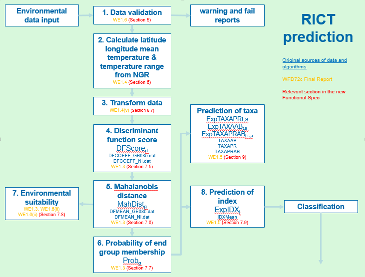
7.2 Prediction Overview

The probability of a site belonging to an End Group is determined by the similarity of its Environmental Variables (EVs) to those of the relevant End Group.

Due to the multivariate nature of the environmental variable data, Multiple Discriminant Analysis (MDA) is used to turn the environmental variable data into a format that can be used to discriminate between the end groups.

MDA depends on multiple Discriminant Functions (DF). A Discriminant Function has the general format:-

Z = constant + c1EV1 + c2EV2 + c3EV3 + ... + cnEVn

where Z is the Discriminant Score (DS) for that particular discriminant function, c1…cn are the coefficients of that discriminant function and EV1…EVn are the values of the environmental variables.

A DF is a linear combination of the EVs and the coefficients, which maximises the separation in data space of the end groups. In other words, if the discriminant function was solved for the mean values of the environmental variables of each end group and the results plotted on a line, the value from the solved formula for each end group would be as far apart from its nearest neighbour as could be achieved by using the available environmental variables to separate the end groups

7.3 Environmental Variables

The values of the EVs relevant to the prediction run will have been determined during the acceptance, validation and subsequent conversion processing of the input data as described in section 5 and 6 of this document. These are referred to in the algorithm below as EnvvN.

7.4 Discriminant Functions and Coefficients

The RIVPACS model used will determine the Discriminant Functions (DFs) that have to be run. For the GB model 1 with 13 EVs the DFs values can be found in the inst/ext folder for GB in a file called DFCOEFF_GB685.

For the GB model 44 with 17 EVs the DFs values can be found in the prediction support files folder for GB in a file called discrimant-function-coefficients-model-44.csv - see section 14 for additional Model 44 information.

For the NI model with 11 EVs, the DFs values can be found in the prediction support files folder for Northern Ireland in a file called DFCOEFF_NI

These are separate occurrences of DF. Each of these has a single ‘constant’ and, for each component EV, a co-efficient that is to be applied to the EV value. The coefficients are referred to in the algorithm below as DFCoef.

7.5 Calculate Discriminant Function Scores

(Step 4 in diagram above)

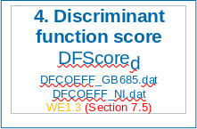
The functions that RICT uses for the calculations in the steps below (steps 4 - 8) can be found in the prediction-functions.R file. The algorithms and definitions provided below are copied from WFD72C and have been used to create the functions.

For each DF, the Discriminant Score needs to be calculated as follows:

DFScore_d = DFCoef_1,d * Env1 + … + DFCoef_vN,d * En_vvN; for d = 1. … dN

Definitions – these have been copied from WFD72C:

v = id of current environmental predictor variable
vN = number of environmental predictor variables
d = id of current discriminant function axis
dN = number of discriminant function axes in current Reference end group set
DFCoef_v,d = discriminant function coefficient for predictor variable v on
discriminant function d obtained from the values in the DFCOEFF_GB685 file for
Great Britain, DFCOEFF_NI file for Northern Ireland or discrimant-function-coefficients-model-44.csv for model 44 which can be found within the prediction support files.
Env_v = value of environmental predictor variable v for the current test site
DFScore_d = discriminant function score on axis d for the current test site

7.6 Calculate Mahanalobis Distance

(Step 5 in diagram above)

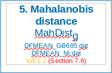
For a particular End Group g, the probability of End Group Membership is calculated as follows:

Calculate Mahanalobis distance (MahDistg) of test site from each End Group

MahDistg = (DFScore1 - DFMeang,1)2 + ... + (DFScoredN - DFMeang,dN )2 ; for g = 1,...,gN

Definitions – these have been copied from WFD72C:

g = id of current end group (set ID: 1 = GB, 2 =NI)
gN = number of end groups in current Reference end group set
NRef_g = number of reference sites in end group g
DFMean_g,d = mean discriminant function score of end group g on axis d Obtained from the ‘target’ values in the DFMEAN_GB685 file forObtained from the table x-103-end-group-means-formatted-jdb-17-dec-2019.csv which is within the inst/ext folder) Great Britain, DFMEAN_NI file for Northern Ireland or end-group-means-discriminant-scores-model-44.csv for Model 44.
MahDistg = Mahalanobis distance of test site from end group g

7.7 Mahanalobis Distance

Use Mahanalobis distance to determine probability of End Group membership (Step 6 in diagram above):

Calculate the PDistg for each End Group

PDist_g = NRef _g * EXP(-MahDist_g/2)

where NRef g = the number of reference sites in the End Group (from the End Group Reference Data table) and EXP is the natural exponential function

Calculate the PDistTot

PDistTot = PDist₁ to PDist _gN

where gN is the number of end groups in the relevant end group set

Calculate the Probability of End Group Membership (Prob_g)

Prob_g = PDist_g / PDistTot

where Probg is the Probability test site belongs to end group g

At the end of this process we end up with a set of probabilities of End Group Membership, one for each End Group. These are referred to below as Prob₁ to Prob_n.

7.8 Determine Environmental Suitability

Determine environmental suitability of the test site for prediction:

(Step 7 in diagram above)

In certain cases it may be calculated that there is a very low probability of the site being in any of the end groups based on the data provided.

In order to highlight this to the user, a calculation is required to allocate an Environmental Suitability code to the site data indicating the probability the site belongs to any end group. The potential codes are:

1 OK
2 < 5%
3 < 2%
4 < 1%
5 < 0.1%

The required calculation uses the Chi-square values (CQ1 to CQ4) which vary per End Group Set as below:

End Group set (ID)	CQ1	CQ2	CQ3	CQ4
RIVPACS IV GB (set 1)	21.02606	24.05393	26.21696	32.90923
RIVPACS IV NI (set 2)	18.307	21.1608	23.2093	29.5883

prediction-functions.R has a function called getSuitabilityCode() which will do this calculation.

The detailed calculation is as follows:

Calculate the minimum Mahanalobis distance (MahDist_min)

MahDistmin = minimum of (MahDist₁,….,MahDist_n)

Calculate the Environmental Suitability Code and Suitability text

If the MahDist_min < value for CQ1 then Suitability Code = 1 and suitability text is >5%

If the MahDist_min >= value for CQ1 and < value for CQ2 then Suitability Code = 2 and suitability text is <5%

If the MahDist_min >= value for CQ2 and < value for CQ3 then Suitability Code = 3 and suitability text is <2%

If the MahDist_min >= value for CQ3 and < value for CQ4 then Suitability Code = 4 and suitability text is <1%

If the MahDist_min >= value for CQ4 then Suitability Code = 5 and suitability text is <0.1%

The output file will provide the user with the Suitability Code and suitability text. The Suitability text gives the user information and warnings about the suitability code calculated.

7.9 Determine the Predicted Values of Indices

(Step 8 in diagram above)

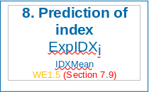
The indices that require to be processed will be identified from the options panel. For the initial release of RICT this will be for WHPT ASPT and WHPT NTAXA sets which are the indices required for the WFD classification. However, for Prediction, all 80 indices (which includes WHPT ASPT and WHPT NTAXA sets), will be used at this point and for Prediction only.

prediction-functions.R contains the following functions which will do this calculation:

rict:::getSeasonIndexScores()

and the: end_group_IndexDFrame uses the x-103-end-group-means-formatted-jdb-17-dec-2019.csv file

Algorithm: (copied from WFD72C)

ExpIDXi = Prob₁ * IDXmean_i,s,1, + … + Prob_gN * IDXmean_i,s,gN

Definitions: (these have been copied from WFD72C)

g = id of current end group
gN = number of end groups in current Reference end group set (set: 1 = GB, 2 =NI)
Prob_g = Probability test site belongs to end group g
i = id of current biological index
iN = total number of biological indices
s = id of selected season(s) combination (referred to as ‘season s’); (1 = spring, 2 = summer, 3 = autumn, 4 = pooled spring + summer, 5 = pooled spring + autumn, 6 = pooled summer + autumn, 7 = all three seasons pooled – only 1, 2 and 3 are used in RICT 2)
IDXMean_i,s,g = Mean value of index i for season s for reference sites in end group g ExpIDX_i = Expected value of index i for selected season s for current test site

Internally-supplied Data files:

A separate file called x-103-end-group-means-formatted-jdb-17-dec-2019.csv will be provides the values for:

IDXMean_i,s,g = Mean value of index i for season s for reference sites in end group g

7.10 Prediction Outputs

Once the prediction processing has been completed, the following data has been calculated for each occurrence of site data:

Probabilities of End Group Membership
Expected Index Values
Predicted Taxa occurrence details

The expected index data is then passed to the classification process.

8 All index prediction

This provides predictions for a wide range of indices.

However, it uses a different end group means data file derived from the RIVPACS database.

The all indices output file will only show the output for prediction for the 80 indices.

The biotic indices included in all index prediction are listed in Appendix B2.

9 Taxa Prediction

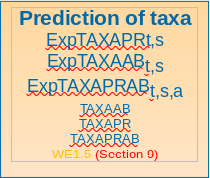
Although not required for status classification, an important feature of RIVPACS that is included in RICT is to be able to predict the taxa expected to be present at the site. For each taxon, the prediction provides:

Expected probability of occurrence.
Expected log abundance category.
Expected numerical abundance.

The steps involved are described below.

9.1 Data Limits

Because of the large amounts data in the output files and stain on the server, the user is limited to 20 sites per run. This restriction is only on the web app. Running the RICT package locally is unlimited.

9.1.1 Taxon prediction data file

All of the required taxon prediction data was supplied by John Davy-Bowker in a single file derived from the RIVPACS Reference Database: TAXA_AB_APR_PRAB.csv

This file contains the following 18 columns:

1. Model                1 = GB, 2 = NI
2. End_Group      1-43 for GB, 1-11 for NI
3. TL                   Taxonomic Level: TL1, TL2, TL3, TL4, TL5
4. Season_Code:     1 = spring, 2 = summer, 3 = autumn

The next 6 columns (5-10) should all be stored as Text columns (even those which appear numeric because they need to retain their leading zeroes.

5. Maitland_Code
6. Maitland_Name
7. Furse_Code
8. Furse_Name
9. NBN_Code
10. NBN_Name

The final 8 columns (11-18) are the 8 parameters whose expected values for any test site we wish to calculate for each taxon at each taxonomic level in each season
  
11. Average_Numerical_Abundance
12. Average_Log10_Abundance
13. Prob_Occurrence
14. Prob_Log1
15. Prob_Log2
16. Prob_Log3
17. Prob_Log4
18. Prob_Log5

Note: For the GB model, at any one taxonomic level (TL1 – TL5) and particular season (1-3), any particular taxon at that level only occurs as a row in this input file if it occurred (i.e. has at least one positive taxonomic parameter value) in at least one of the GB RIVPACS IV reference site End-groups. Similarly for taxa in the NI model. Thus the taxa listed (i.e. given) rows varies slightly between seasons because not all taxa were found in every seasons in at least one of the RIVPACS IV model reference sites.

TL1 = BMWP taxa
TL2 = WHPT taxa
TL3 = all RIVPACS families
TL4 = all RIVPACS species
TL5 = mixed taxon level

Season 1 = spring, 2 = summer, 3 = autumn.

9.1.2 Calculate Expected for a GB test site

End-group means of the 8 parameters to be predicted are supplied in columns 11-18 of the above taxon prediction data file.

When working on the GB model, you first need to subset the data in the taxon prediction file to eliminate the rows for NI (Model =2).

Assuming the RICT software has already read the test site’s environmental input data and calculated the probabilities (P1 , P2 , … P43) of the test site belonging to each of the 43 GB Model End-groups, for any particular taxa K at taxonomic level L in season S, its predicted expected value (ExpJKLS) of Taxonomic parameter J for that season is given by:

E_JKLS = P1 x M_JKLS(1) + P2 x M_JKLS(2) + … + P43 x M_JKLS(43)

Where M_JKLS(i) = supplied End-group mean of taxonomic parameter J of taxa K at taxonomic level L in season S.

In a mathematical sense that’s it and it appears easy. However, in practice it is not easy, not only because of the vast number of taxa, taxonomic level, end-group and season combinations for which Expected values are required, but also because the number of taxa included in the input file varies between seasons.

9.1.3 Calculate all taxonomic expected values

The following computing trick calculates the expected values of taxonomic parameters for all taxa at all levels in all seasons in one step.

If (P₁ , P₂ , … P₄₃) denote the probabilities of the current test site belonging to each of the 43 GB Model End-groups, then:

Copy column 2 (‘End_Group’) to a new column ‘End_Group_Prob’
Use a software coding (translation) function to recode the new ‘End_Group_Prob’ column so that : 1 becomes P₁ , ₂ becomes P₂, … , 43 becomes P₄₃
For any particular taxonomic parameter J (denoted here ParamJ and supplied in one of columns 11-18), calculate new column ParamJ_Prob as:

ParamJ_Prob = End_Group_Prob  x ParamJ

Use a software multi-way table function using columns (4, 3, 7, 5, 6, 8, 9, 10,) in that order as multi-way table classifiers and then sum the column ‘ParamJ_Prob’ across all 43 ‘End-groups’ which it will do by default in any sum function as ‘End_Group’ is not one of the table classifiers.
You actually want to use a multi-way table function which creates a new output set of columns with one new column for each table classifier and one for the sum across end-groups of the column ‘ParamJ_Prob’
In fact, if you can do this for one of 8 taxonomic parameters, you could probably do it for all 8 parameters at one step, having first derived the 8 intermediary columns: Param1_Prob, Param2_Prob,… , Param8_Prob

The order of multi-way table classifying columns that I specified above, namely (4, 3, 7, 5, 6, 8, 9, 10) will ensure that new columns of Expected taxonomic parameters will have classifier columns sorted first on Season, then Taxonomic Level, then Furse code, and finally all of the other alternative taxonomic codes for a taxa. I have suggested using ‘Furse_Code’ as the first (and primary individual taxonomic code) as I think it is unique and always available. It will also make it easier to compare with Ralph’s independent test code.

In summary, this should lead to an output file of 18 columns, akin to those in the input file, but where the values in output file columns 11-18 are now the predicted Expected values for the 8 taxonomic parameters for each combination of season, taxonomic level and taxa code as specified in output file columns 1-10.

This procedure could be done for each test site in turn. The 18 output columns for each site could be stacked so that there is one additional output column denoting ‘SiteName’.

The single output file of columns can now be re-sorted externally by the User or use to subset by SiteName, Season, Taxonomic Level and/or Tax code, as required. For example, to just get predictions of taxonomic parameters for taxa at taxonomic level TL1 (BMWP family level), you just subset the 18 output columns by column TL= TL2.

If the user wishes to only view the prediction results, a csv output will be generated which can be downloaded and used for reports.

9.1.4 Taxon prediction Output

Taxon prediction output includes a row for each taxon predicted. For each site, expect about 3500 rows of data. The first block of rows will be for the first site selected and below it the results for the second site. Each row includes the same columns as the taxon prediction data file, together with siteName. Sections below are based on notes from write up with Maybin (March 2020):

9.2 Data Input files

9.2.1 GB & NI

New Input File: New_Input_file_Data_to_use_multi_year.csv
prediction-functions.R
helper-functions.R

9.3 R code for taxa prediction

The rict_predict function this is the same as previous predictions but for taxa prediction we need to find each site’s EndGroup, it uses columns 15:57 for GB and 13:23 for NI.

An important file as it looks at the taxonomic info from the TAXA_AB_APR_PRAB.csv about the model to be used in the prediction. EndGroup found are used with this file to compute predictions.

If the argument taxa = TRUE the function loops through each site and processes each site to do the predictions.

10 Classification

10.1 Classification Process Summary

The flow diagram below summarises the classification process and calculations as well as identifying the relevant section for further information from the WFD72C final report and other sources of information:

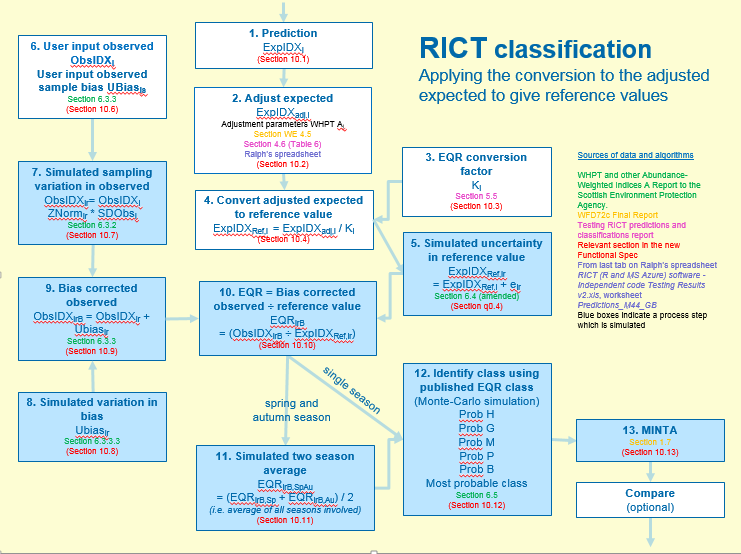
Note that the blue boxes indicate processes that are simulated.

10.2 Classification overview

For every site in the input to the classification process consists of Observed and Expected Index Values for the ‘current year’ for each applicable index.

Multiyear classification will include Observed and Expected Index Values for up to two previous years for each applicable index.

For the WFD classification, RICT will use TL2 WHPT Abundance weighted with distinct taxa for ASPT and NTAXA indices.

Any functions that RICT uses for the calculations described in the steps below (steps 1 - 13), can be found in the ClassificationfunctionsV2 within the classification support files folder. The algorithms and definitions provided below are copied from WFD72C plus other sources and have been used to create the functions.

10.3 Calculate Expected Values

(Step 1 in process diagram above and Section 7)

This is the main result from RIVPACS prediction (Section 7), based on environmental variable data input by the user. It is the prediction of the value of the index expected at the site if it was in the best quality available for that type of site, based on samples collected from best available reference sites.

10.4 Adjust Expected Values

(Step 2 in process diagram above)

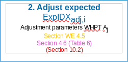
The aim of this step is to standardise the raw predictions so that they relate to the same environmental quality (the high/good boundary quality) using algorithms first developed in WFD72b. This step is necessary to take account of variation in the environmental quality of RIVPACS reference sites.

There are a number of processes involved in this step as described below:

The computeScoreProportions() function within the prediction support files folder is used to calculate proportions (Qij) for each end group using a CSV file (also within the prediction support files folder) called EndGrp_AssessScores.
The getWeighted_proportion_Rj() function within the prediction support files folder is used to calculate weighted proportions (Rj) using the probabilities from prediction process by multiplying with the Qij proportions.
The compute_RjAj() function within the prediction support files folder is used to calculate RjAj by multiplying the weighted proportions by the adjustment factors. See below for details regarding the adjustment factors.
Finally, the RjAj value is used to divide by for all the predictions (NTAXA and ASPT) to get the adjusted expected value (ExpIDXadj,i) for each site and each index.

The reference adjustment values referred to above are default values for the WFD classification and can be found in adjustParams_ntaxa_aspt csv file within the classification support files folder.

This supporting data table csv file contains the number of reference sites by Biologist assessment score (1-5) for each End Group together with the five adjustment factors (Q1, Q2, Q3, Q4, Q5) for each index.

The source for this csv file is based on the Table 6 from the Testing RICT predictions and classifications draft report 2018 which is as below:

Index	WHPT NTAXA	WHPT ASPT
Q1	1	1
Q2	1	1
Q3	1	1
Q4	0.967	0.977
Q5	0.926	0.945

Table 1. Adjustment factors for reference site quality (Q1, Q2, Q3, Q4, Q5) for abundance-weighted WHPT NTAXA and WHPT ASPT

However, further work has been done which has resulted in slightly different values for these adjustment factors which are reflected in the adjustParams_ntaxa_aspt.csv file used by RICT, It is expected that the Testing RICT predictions and classifications draft report 2018 will be shortly updated to include a Table 7 to show these changes.

There is one set of adjustment factors for each index. Within current RICT, adjustment factors for WHPT NTAXA and WHPT ASPT have been calculated.

10.5 EQR Conversion Factor

(Step 3 in process diagram above)

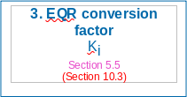
This is the conversion factor used to convert the adjusted predictions that relate to high/good boundary quality to reference values that relate to reference condition, which is somewhere in high status (reference values are the average value of the metric at reference sites in reference condition = high status)

Each index has a different conversion factor, based on the average value of the index at all RIVPACS Reference Sites divided by the value at RIVPACS reference sites that are in WFD high status (reflected in Biologists’ Assessment values for each reference site).

For the default WFD classification in RICT the conversion factor value will be (as copied from Section 5.5 of the Testing RICT predictions and classifications draft report 2018):

1.0049 for WHPT NTAXA
0.9921 for WHPT ASPT

10.6 Convert adjusted expected to reference value

(Step 4 in process diagram above)

The aim of this step is to convert the predictions from high/good boundary to reference values, which is somewhere in high status (actually the average value of the index at reference sites in high status), by applying the conversion factor.

The conversion factor is applied to the adjusted expected value to give an expected reference value which will be used to calculate the EQRs expected by the Water Framework Directive.

Specifically, ExpIDXRef,i is calculated as:

ExpIDX_Ref,i = ExpIDX_Adj,i / K

Where:

ExpIDX_Adj,i = value which is calculated as described in Adjust Expected Values section.
K = WFD conversion factor (i.e. WHPT NTAXA: K = 1.0049, and WHPT ASPT K = 0.9921 as described in EQR conversion Factor section.
IDX = do this for each Index, i.e. for WHPT NTAXA and WHPT ASPT
i = do this for each specific site

This avoids the need for the intermediary step of calculating and referring to EQI (Environmental Quality Indices) values (which are calculated as EQI = Obs / ExpAdj) and means that the site classifications can use the published class limits for index EQR values directly.

This calculation is done directly within RICT code and not via any function.

10.7 Simulate uncertainty in expected

(Step 5 in process diagram above)

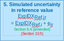
The aim of this step is to take account of error in measurement of environmental variables used to predict the reference values.

It should be noted that the “ +eir “ shown in the algorithm in the process step above is a summary of the algorithm values of ZExpir * SDExpi / √(NExpyear) as described in further detail below. It is the error term used to adjust the expected value.

The simulation of uncertainty in ExpRef is obtained using the algorithms in Section 6.4 of the Clarke & Davy-Bowker WHPT indices RICT Report of March 2014 report, but now where uncertainty in the Expected values is measured about the WFD Reference-adjusted value ExpRef., this has been amended as described below.

Main algorithm used:

ExpIDXir = ExpIDX_i + ZExp_ir * SDExp_i / √(NExp_year)

Where (using the same notation as section 6.4 of the 2014 WHPT report):

ExpIDX_i = WFD Reference-adjusted Expected value (ExpRef) of index i
ExpIDX_ir = WFD Reference-adjusted Expected value of index i in simulation r
SDExp_i = Error SD for expected value of index i
NExp_year = 1 for single-year run
= number of years (1, 2 or 3) for which a separate estimate of the E value was involved in the estimate of average E value (for multi-year run)
ZExp_ir = Random number deviate from a standard Normal distribution with a mean of 0.0 and SD of 1.0, for use in simulation r for index i

Where:

SDExp₇ = 4.3 = Measurement error SD of Expected values of weighted WHPT Score (index 7)
SDExp₈ = 0.53 = Measurement error SD of Expected values of weighted WHPT NTAXA (index 8)
SDExp₉ = 0.081 = Measurement error SD of Expected values of weighted WHPT ASPT (index 9)

Within RICT, these calculations are done using functions which can be found in the ClassificationfunctionsV2 (within the classification support files folder).

It should be noted that it is important to do this for each index and also be aware of the numbering for each index. As indicated above, each index has a number, i.e.:

WHPT Score (index 7)
WHPT NTAXA (index 8)
WHPT ASPT (index 9)

10.8 Calculate Bias Adjustment

(Step 6 in process diagram above)

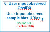
RICT classification requires users to input an observed value for an index (ObsIDXi), based on samples collected in the field. This value is provided by the user completing the relevant data field in the input file as described in section 5 and Annex B of this document. Values are required for each index and for all three seasons, spring, summer and autumn.

Users may also input a bias value (UBiasis) for NTAXA, which reflects the impact of analytical error (measured by auditing) on the observed index values. This value is provided by the user completing the relevant data field in the input file as described in section 5 and Annex B of this document. RICT calculates bias for ASPT from bias for NTAXA and the observed NTAXA. If no input value for Bias is provided, RICT will use a default value of 1.68.

If bias correction is not wanted, users should enter a bias value of zero into the relevant data field in the input file. The zero value must be entered and not left blank or RICT will use a default value.

10.9 Simulate uncertainty in observed values

(Step 7 in process diagram above)

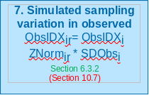
These simulations take account of sampling error, estimated in replicated sampling studies, including the Biological Assessment Methods Study (BAMS) which is needed so that statistical confidence of the status classification can be estimated.

The main algorithm used:

ObsIDX_ir = ObsIDX_i ZNorm_ir * SDObs_i

Where:

ObsIDX_i = input value provided by the user for observed value for an index
ZNorm_ir = Random number deviate from a standard Normal distribution with a mean of 0.0 and SD of 1.0 for index i in simulation r
SDObs_i For single-year runs: SDObs_i = √( (SDRep_i)² + (SDTSeas_i)²)
Where values for SDRep = 0.269 and SDTSeas = 0.279
Definitions for each index used within RICT (which are only the abundance-weighted WHPT indices are as below copied from Section 6.3.3.2 (b) of the WHPT and other Abundance-Weighted Indices SEPA Report:
ObsIDX8r = (√(ObsIDX8) + ZObs8r)² = rth simulated value for observed weighted WHPT NTAXA
ObsIDX9r = ObsIDX₉ + ZObs_9r = rth simulated value for observed weighted WHPT ASPT
ObsIDX7r = ObsIDX_8r * ObsIDX_9r = rth simulated value for observed weighted WHPT Score

Within RICT, these calculations are done using functions which can be found in the classification-functions.R.

10.10 Simulate variation in Bias

(Step 8 in process diagram above)

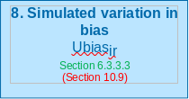
This is simulation of user input bias which is calculated in RICT using the getUbias8r() function found in the classification-functions.R.

The algorithms used within this function are as below which is copied from Section 6.3.3.3 of the WHPT and other Abundance-Weighted Indices SEPA Report.

Definitions

ObsIDX_ir = Simulation r Observed sample value of index i for current test site (uncorrected for bias)

Ubias₈ = estimate of average net under-estimation of WHPT NTAXA for the observed sample

Ubias₈ is either:

input by the user of the RICT software
estimated as 36% higher than the user-input bias (Ubias2) for number of BMWP taxa i.e. Ubias₈ = 1.36 Ubias₂

Ubiasir   = Estimate of bias (net under-estimation) of index i for simulation r
ObsIDXirB = Bias-corrected observed value of index i for simulation r

Special case: when no WHPT taxa were recorded in the sample (i.e. ObsIDX8 = 0), assume none were missed (i.e, set Ubias8 = 0)

Ubias_8r = bias (net under-estimate of number of WHPT taxa) for simulated sample r, estimated as a random deviate from a Poisson distribution with a mean of Ubias₈

Zbias_9r = Random number deviate from a standard Normal distribution with a mean of 0.0 and SD of 1.0

Ubias_9r = abundance-weighted WHPT ASPT of the Ubias8r missed WHPT taxa for simulated sample r

= u_9a + u_9b * ObsIDX₉ + Zbias_9r * (u9c / √Ubias_8r)

where u_9a = 4.35 , u_3b = 0.271 , u_9c = 2.5

Then:

Ubias_7r = Ubias_8r * Ubias_9r = bias of abundance-weighted WHPT score for simulated sample r

10.11 Correct observed values for bias

(Step 9 in process diagram above)

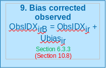
The aim of this step is to use the values provided in the previous steps, add them together to give an overall calculated observed value corrected for Bias. Bias is a measure of the impact of laboratory error on the value of observed indices. It is calculated from audits of laboratory performance and is input by users as described in Calculate Bias Adjustment section above.

The main algorithm used is:

ObsIDX_irB = ObsIDX_ir + Ubias_ir

Where:

ObsIDX_irB = Bias corrected observed value
ObsIDX_ir = Simulated observed value from Simulate uncertainty in observed values section above
Ubias_ir = Simulated Bias value from Simulate variation in Bias section above

Within RICT, these calculations are done using functions which can be found in the ClassificationfunctionsV2 (within the classification support files folder).

The algorithms used within this function are as below which is copied from Section 6.3.3.3 of the WHPT and other Abundance-Weighted Indices SEPA Report.

ObsIDX_7rB = ObsIDX_7r + Ubias_7r = bias-corrected observed abundance-weighted WHPT Score for simulation r
ObsIDX_8rB = ObsIDX_8r + Ubias_8r = bias-corrected observed abundance-weighted WHPT NTAXA for simulation r
ObsIDX_9rB = ObsIDX_7rB / ObsIDX_8rB = bias-corrected observed abundance-weighted WHPT ASPT for simulation r

It should be noted as mentioned previously, that it is important to do this for each index and also be aware of the numbering for each index. As indicated above, each index has a number, i.e.:

WHPT Score (index 7)
WHPT NTAXA (index 8)
WHPT ASPT (index 9)

Optionally, the simulated EQRs are stored for each metric at this point if required for Compare.

10.12 Calculate Environmental Quality Ratio (EQR)

(Step 10 in process diagram above)

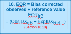
The aim of this step is to express the observed value of the index as an indication of human impact by removing the effect of natural environmental conditions.

Status class boundaries for WFD are expressed as EQRs.

Simulated EQRs, based on simulated observed and expected values, are needed to estimate probabilities of class.

The main algorithm used is:

(EQRirB = (ObsIDXirB ÷ ExpIDX_Ref,ir)

Where:

EQR_irB = simulated bias-corrected EQR value for index i

ObsIDX_irB = Bias-corrected observed value of index i for simulation r as calculated in Correct observed values for bias section.

ExpIDX_Ref,ir = Reference-adjusted Expected value of index i in simulation r as calculated in Convert adjusted expected to reference value section.

This calculation is done directly within RICT code and not via any function.

10.13 Combine spring and autumn EQRs

(Step 11 in process diagram above)

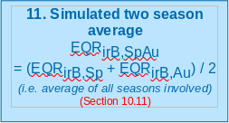
The aim of this step is to increase precision of classification and take account of seasonal variations in environmental quality.

The WFD status must be based on EQRs calculated from spring and autumn samples. These values must be calculated and available for this step to calculate the seasonal average.

The EQR values for spring and autumn samples are divided by the number of season (i.e. 2) to calculate the seasonal average for each simulation. The main algorithm is:

EQR_irB,SpSuAu = (EQR_irB,Sp + EQR_irB,Au) / 2

Where:

EQR_irB,SpSuAu = Season average EQR

EQR_irB,Sp = EQR value for spring season refer to Calculate Environmental Quality Ratio (EQR) section

EQR_irB,Au = EQR value for autumn season refer to Calculate Environmental Quality Ratio (EQR) section

This is calculated in RICT using the getAvgEQR_SpAut() function found in the classification-functions.R (within the classification support files folder).

10.14 Determine the probability of the class

(Step 12 in process diagram above)

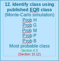
The aim of this step is to take account of imprecision in monitoring data in the classification.

The probability of each class is simply the sum of the simulations resulting in that class and is included in the output file.

As copied from Section 6.5 of the WHPT and other Abundance-Weighted Indices SEPA Report:

“Confidence of class - The likelihood of the true status class (i.e. averaged across all possible samples) of a test site being each of the five possible WFD classes is estimated simply by applying the ‘status classification method’ to each simulation sample r in turn. Thus the class for simulation r is based on the EQI/EQR values for simulation r, namely the set of EQIir. For each index and overall, the proportion of simulations assigned to a status class estimates the probability that the true (average) quality of the test site for that time period was of that ecological status class (based on its macroinvertebrates).”

So to summarise, the probability of each class is simply the sum of the simulations resulting in that class and this data is calculated and then included in the output file.

10.15 Determine the worst overall class

(Step 13 in process diagram above)

The aim for this step is to ensure that the classification reflects ecological impacts caused by any type of environmental pressure.

The overall status class for a sample is defined to be the worst of classification based on number of taxa and ASPT. This is referred to as the MINTA class (i.e. MINimum of classes based on number of Taxa and ASPT).

The WFD status of a site or water body is based on the worst class indicated by either WHPT ASPT or WHPT Ntaxa, following the ‘one out all out’ rule.

The WFD requires that all water bodies, including rivers sites, are classified into one of five ecological status class. These classes in RICT are coded as classes 1-5 with 1= ‘high’, 2=‘good’, 3=‘moderate’, 4=‘poor’ and 5=‘bad’.

There are a number of processes involved in this step as described below:

The EQR values calculated above are used within the getClassarray_ntaxa() and getClassarray_aspt() function found in the classification-functions.R to find the class and relevant boundary limit values.
The getMostProbableClass() function found in the classification-functions.R is used to find the most probable class.
The getMINTA_ntaxa_aspt() function found in the classification-functions.R is used to find the maximum of the two classes and which is the worst class. The worst class in then recorded in the output file and displayed in the MINTA column

10.16 All Season Outputs

For Isle of Man classification, an additional output is calculated which includes an extra 19 columns for ‘all seasons’ outputs. This feature provides outputs for ASPT, NTAXA and Minta outputs for all seasons present in a particular row in the input file. For instance, if summer and autumn observations are in the first row of the input file, these will be classified in the ‘all_seasons…’ columns. Likewise, if Spring and Summer and in the next row of the input file, this will be combined in the ‘all seasons…’ output. If a single season is provide, this will also be reported in the ‘all_seasons’ columns. Additionally, if Spring, Summer and Autumn are provided. In other words, any combination season(s) observations provided in the input file will be reported in the ‘all_seasons…’ columns.

See Annex B All Seasons for example of the output.

This provides the ability to classify different combinations of seasons not just Spring and Autumn as required for WFD classification.

10.17 Classification output

An output file will be created to show the calculated data results for prediction and classification. The output file will also indicate any validation errors found during the run and specify which values resulted in either a “fail” or “warn”.

The output file will be in csv format to be downloaded by the user and used for reporting. There will be an output file available for prediction and an output file available for classification.

11 Multi Year Classification

The aim of multi-year is to take account of temporary differences in quality and improve precision if a user has more than one year of sample data.

River Invertebrate status must be assessed every 3 years for WFD. Where sites are sampled in a 3 year monitoring cycle, WFD status can be based on samples collected in more than one year.

Multi-year status classification takes account of inter-year variation based on observations from specific rivers and streams.

The multi-year classification will need to following:

Assessment is always on a 3 year period.
Users may supply 1, 2 or 3 years data.
A complete year’s data must include spring and autumn – otherwise this year cannot be included in the assessment.
Therefore minimum requirement is 1 year of data which includes spring and autumn.
Each year will be added as a separate row on the input file and for each year of data will have the same site name
RICT will check each row to see if it is same site name, if it is will store the simulations and include this in the assessment and will carry out this check for the next row to collect a maximum of 3 years of data.
There will be no changes needed to the input file as the user will select the multi-year option.
Ralph will be able to obtain some test data which can be used to clarify if the calculations are correct.
Output file will need to be amended to display the multi-year data and will display the term “multi-year” instead of the actual year in the Year column.
Apart from the differences highlighted above, the multi-year classification will follow the same process at the Prediction and Classification procedures specified in the previous sections of this document.

We assume simple averaging based on the same number of samples involved in each year, but not necessarily the same seasons. There is therefore no problem (from a statistical point of view) if spring one year and autumn the next, but we do have a problem if year 1 = single season and Year 2 = 2-season classification. Basically, we assume the same sampling effort each year. However, remember that official WFD status classification must always be based on 2-season spring + autumn data.

12 Multi-site classification

The aim of multi-site classification is to determine the overall status class for a water body based on samples collected from more than one site. The Environment Agency collects samples from some water bodies from more than one site.

The Environment Agency currently uses VISCOUS software to calculate WFD status for water bodies monitored from more than one site, as well as sites sampled in more than one year before 2019. Multi-site will allow the Environment Agency to replace VISCOUS completely, and therefore streamline the classification process.

Multi-site classification uses similar algorithms to multi-year classification. Additionally, its output indicates which sites have been used.

As with multi-year, we assume simple averaging based on the same number of samples involved in each year within the water body (not necessarily the same seasons). There is therefore no problem (from the point of view of multi-year classification) if spring one year and autumn the next, but we do have a problem if year 1 = single season and Year 2 = 2-season classification. Basically, we assume the same sampling effort each year. However, remember that official WFD status classification must always be based on 2-season spring + autumn data.

13 Compare

The relevant parts of the algorithms section of the SNIFFER WFD72C project 2008 Final Report have been extracted and adapted here to explain the algorithms needed to code the Compare procedure in R.

The new RICT only refers to EQR values (which are bias-corrected observed (Obs) values divided by WFD reference-adjusted Expected (ExpRef) values, all WFD72C algorithms section references to former EQI (Obs/Exp) values are replaced by their new counterpart EQR values to improve explanation of how to program the new RICT Compare procedure.

Compare flow chart:

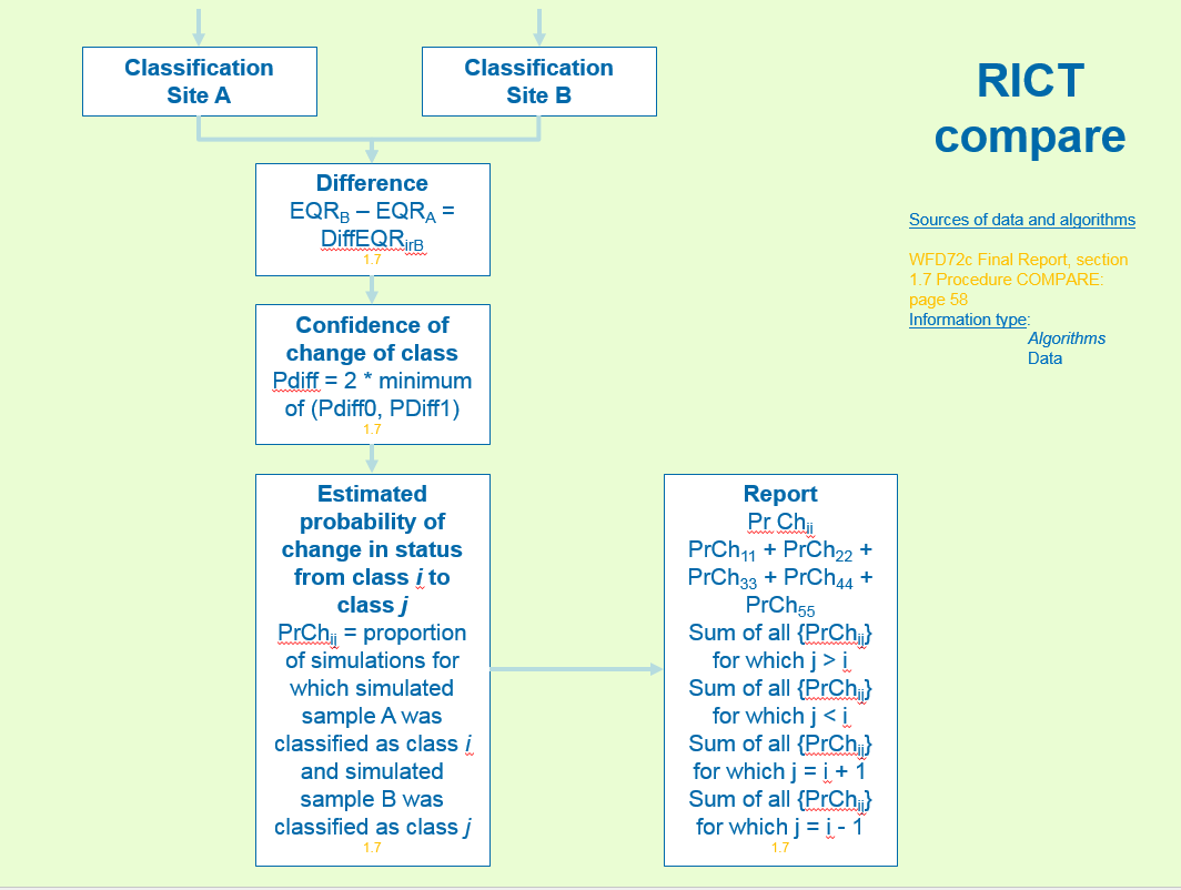
The Compare procedure allows the user to assess whether there is a real difference in EQR values and/or status class between a pair of samples and/or sites and/or time periods. This is done using an extension of the simulation techniques and algorithms described above that are used to assess the EQRs and ecological status class and the associated uncertainty for individual samples/sites and time periods.

The first sample in a pair is known as result A and the second as result B.

In each simulation r, independent simulated EQR values are calculated for each index i for each of the two results. Correct observed values for bias. In this context, independent simulations means that the various random uncertainty terms are different and completely independent for the two simulated samples A and B for any simulation r.

To compare results, the two input files into Compare must contain the same number of rows. The two files are then compared pair-wise, row to row for each result. For instance, if comparing a single upstream result to multiple downstream results, repeat the single result over multiple rows (equal to the number of downstream results) in the input file.

Note, Compare allows individual-season estimates of class for spring and autumn to be compared.

Calculate Difference and Related Statistics:

Average EQR for Results A = mean(EQR_A)

Average EQR for Results B = mean(EQR_B)

Average EQR: Difference (B- A) (DiffEQRirB) = EQR_B – EQR_A

For each simulation r, the difference in the two simulated EQR values (sample B value minus sample A value) is calculated for each index i to give DiffEQRirB when corrected for bias.

Standard Deviation of Difference = SD of the rN simulated values of EQI_i (corrected for bias) for index i for the current test site

Calculate the SD, (SDEQR_i) of the rN values of EQR_ir in the usual way for calculating any SD.

Lower 95% (L95) of Difference = Lower 2.5 percentile of the rN simulated values (EQR_ir) of EQR (corrected for bias) for index i for the current test site

Upper 95% (U95) of Difference = Upper 2.5 percentile of the rN simulated values (EQR_ir) of EQR

Determine the lower and upper 2.5 percentiles and thus 95% confidence limits by sorting all of the rN simulated EQRir values into order from smallest to largest. Then the lower and upper percentiles are given by the mL and mU smallest values, where:

mL = nearest integer to 0.025 * (rN + 1)

mU = nearest integer to 0.975 * (rN + 1)

For the recommended rN = 9999, mL = 250 and mU = 9750.

Confidence (and statistical test) of change/difference in EQR:

Confidence limits for the difference in EQR values are obtained from the frequency distribution of the differences (DiffEQRir) using the same approach as for single sample EQR values described above, namely, order the differences from smallest to largest and find the 2.5 and 97.5 percentile values of the order distribution.

Strictly speaking we can’t do a normal type of statistical test for the statistical significance of the difference (DiffEQRir) in EQR because we only actually have one sample on each occasion with no actually replication. However, we can generate a type of statistical test using the simulated EQI values, or more specifically, the frequency distribution of the simulated differences (DiffEQRir).

PDiff0 = proportion of simulated differences less than or equal to zero.

PDiff1 = proportion of simulated differences greater than or equal to zero.

2-sided test probability p of No difference in EQR (PDiff) = 2 * minimum of (PDiff0, PDiff1)

Then PDiff is the two-sided test probability of the null hypothesis of no difference in true EQR values between the sites and/or times from which the two samples were taken. [True EQR for a site, in this sense, means average EQI amongst all possible samples from the sites as estimated from the simulated values of EQR].

Code to calculate the difference and related statistics can be found in the compare_test() function. Note, that the simulated EQRs are randomly re-ordered (using set.seed). This is because the simulate EQRs are created in the rict_classify() using the same set.seed and will have equal variance add to each simulated EQR. Therefore, if we calculate the difference without re-ordering the result will be zero. In other words, the difference will cancel out. By re-ordering, we ensure the there will be a difference for each pair of EQRs compared.

Confidence of change in status class:

Each of the two simulated samples is assigned to a status class by applying the ‘status classification method’ independently to the simulated EQR values for each sample for that simulation. This is done repeatedly in rN simulations to build up a two-way frequency (and hence probability) distribution that the site (in its time period) from which sample A was taken was of status class ‘x’ (say) and the sites (in its time period) from which sample B was taken was of class ‘y’.

From this two-way probability distribution, the probability that samples A and B are from the same quality band can be estimated, together with the probabilities that sample B is one band better than A, one band worse, two or more bands better, or two or more bands worse.

In terms of RICT software, a 5 x 5 probability tables of changes is calculated internally using compare_probability() function. This is done for each index for which class limits are to be used and for each multi-index MINTA classification method.

In each case, a wide range of outputs are derived from this table and presented to the user as listed below.

If for coding purposes classes ‘high’ to ‘bad’ are referred to as classes 1-5 respectively, then

PrChij = Proportion of simulations for which simulated sample A was classified as class i and simulated sample B was classified as class j.

= Estimated probability of change in status from class i to class j

	Status class of sample B
		high (1)	good (2)	mod (3)	poor (4)	bad (5)
Status class of sample A	high (1)	PrCh₁₁	PrCh₁₂	PrCh₁₃	PrCh₁₄	PrCh₁₅
	good (2)	PrCh₂₁	PrCh₂₂	PrCh₂₃	PrCh₂₄	PrCh₂₅
	mod (3)	PrCh₃₁	PrCh₃₂	PrCh₃₃	PrCh₃₄	PrCh₃₅
	poor (4)	PrCh₄₁	PrCh₄₂	PrCh₄₃	PrCh₄₄	PrCh₄₅
	bad (5)	PrCh₅₁	PrCh₅₂	PrCh₅₃	PrCh₅₄	PrCh₅₅

Find the most frequent class (random pick if equal frequency across two or more classes):

Most* Probable Class for Result A = most frequency class (status classification method(EQRA))

Probability of most likely class for Result A = Proportion in most probable class

Probability of most likely class for Result B = most frequency class (status classification method(EQRB))

Probability of most likely class for Result B = Proportion in most probable class

Probability status class of result(s) from which results A and B were taken is:

Both status class i = PrChii

Probability B more than one class Worse than A = sum of all { PrChij } for which j > i + 1

Probability B one class Worse than A = sum of all { PrChij } for which j = i + 1

Probability B same Class as A = PrCh11 + PrCh22 + PrCh33 + PrCh44 + PrCh55

Probability B one class Better than A = sum of all { PrChij } for which j = i – 1

Probability B more than one class Better than A = sum of all { PrChij } for which j < I - 1

Furthermore – extract each output from probability table in this order:

Probability Result A in High & Result B in High
Probability Result A in High & Result B in Good Probability Result A in High & Result B in Moderate
Probability Result A in High & Result B in Poor
Probability Result A in High & Result B in Bad
Probability Result A in Good & Result B in High
Probability Result A in Good & Result B in Good
Probability Result A in Good & Result B in Moderate
Probability Result A in Good & Result B in Poor
Probability Result A in Good & Result B in Bad
Probability Result A in Moderate & Result B in High
Probability Result A in Moderate & Result B in Good Probability Result A in Moderate & Result B in Moderate
Probability Result A in Moderate & Result B in Poor
Probability Result A in Moderate & Result B in Bad Probability Result A in Poor & Result B in High
Probability Result A in Poor & Result B in Good
Probability Result A in Poor & Result B in Moderate
Probability Result A in Poor & Result B in Poor
Probability Result A in Poor & Result B in Bad
Probability Result A in Bad & Result B in High
Probability Result A in Bad & Result B in Good
Probability Result A in Bad & Result B in Moderate
Probability Result A in Bad & Result B in Poor
Probability Result A in Bad & Result B in Bad

Pivot all calculated variables (in bold above) to give one column per variable. Each row represents a pair of classification results.

14 Model 44 Prediction and Classification

The Centre for Ecology and Hydrology (CEH) have produced a database of GIS environmental variables data for every 50m of steam or river for use with the new RIVPACS GB Model M44. T

This database will have a map-based location checker, to enable users to check that the Ordnance survey grid reference that they enter returns data for the catchment that they intended. Many monitoring sites are at the downstream end of rivers close to tributaries, so small error in the grid reference or GIS river line can cause the system to return data for the wrong river, and the database holds data only for one river within each 50m grid. The database holds all the environmental data for Model 44, derived from GIS, including discharge category but not including alkalinity.

This database has been hosted by Add details here

This model produced by Ralph Clark and John Davey Bowker and based on these predictive variables is detailed in the report ‘GIS Re-calibration of the hydromorphology-independent RIVPACS predictive model (M37): new model M44’.

RICT will be used with the new RIVPACS Model 44 to give better predictions of streams impacted by siltation due to flow alteration.

The majority of the coding that has been done in RICT for prediction and classification will also be suitable when running Model 44 prediction and classification.

With minor adjustments, the RICT prediction and classification code is suitable for running both Model 1 and Model 44.

The main areas of development involved understanding how to extract the data from RIVPACS and to link to a location checker as outlined in the picture below:

14.1 Model 44 Validation

The GIS input file spreadsheet may be needed for these values (tbc). However, it should be noted that these values will be provided by the model and not entered by a user.

Detailed validation requirements for model 44 are outlined in the acceptance and validation - section 5 of this document.

14.2 Discriminant function scores

Another difference is that there are now 17 discriminant function scores and discriminant function end group means scores rather than 13. See supporting files:

discrimant-function-coefficients-model-44.csv
end-group-means-discriminant-scores-model-44.csv

14.3 Summary diagrams

The flow diagram below summarises the prediction process and calculations as well as identifying the relevant report for further information:

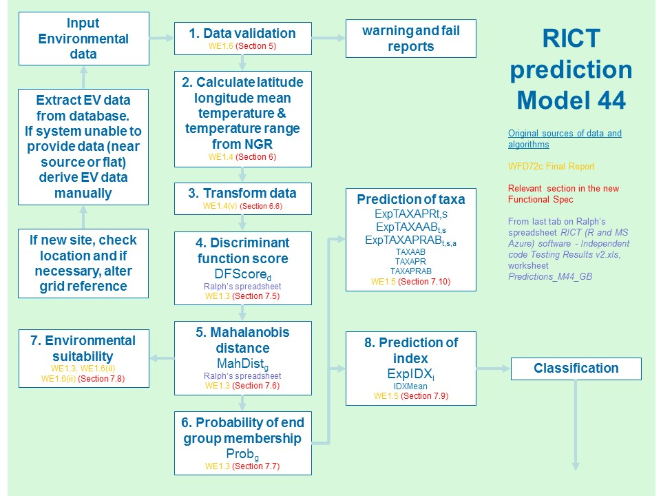
The flow diagram below summarises the classification process and calculations as well as identifying the relevant report for further information:

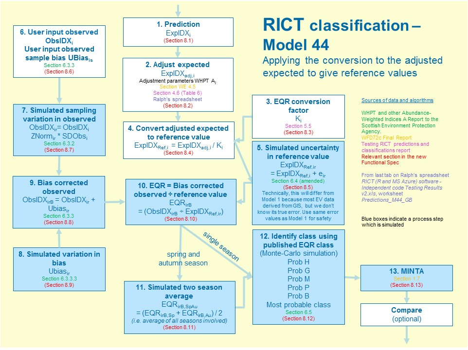
15 Non-Functional Requirements

15.1 Operational Support

The tool needs to be freely available for anyone to access online.

User support for EA users will be via the Defra service desk (at Tier 4 service level) who will route the issue to the appropriate team to deal with. This routing could be to RICT support email or to the Environmental systems team depending on the nature of the issue. EA users will also be able to access an article in MyIT which will provide FAQs to help users with common issues.

User support for other UK regulatory agency users will be via the support email box called RICT support.

There will be no official contracted support for external users but they can send issues and comments to the RICT support inbox

15.2 Look and Feel of User Interface

The user interface will provide intuitive and ‘user friendly’.

15.3 Input and Output Files

Input files will be a standard template in Excel which can be downloaded, completed by the user and then uploaded as a CSV file to RICT. A user guide will be available to help users understand and complete the input file.

The output file will be produced by RICT as a CSV file following the run. A CSV file can easily be opened in Excel or other applications to view the results.

15.4 Hosting

RICT web app is cloud hosted by Posit. The code is hosted on Github.

15.5 Accessibility

Access to RICT functionality may be required by a number of different device types. RICT will be use-able at a minimum by the following device types (model not specified):

Desktop
Laptop

Access to RICT functionality may be required by a number of different browser types. RICT will be use-able in the following browser types:

Chrome
Firefox
Edge

Users will only have access to their own data and cannot access data input or output from other users.

15.6 Performance

RICT will be accessible by multiple concurrent users at any one time without degradation of performance or limitation of features. Users will be internal EA, other UK regulatory body users (SEPA, NRW and NIEA) and external users.

RICT will be capable of processing the prediction and classification of a very large number of sites (approx. 5,000) once per year.

RICT will meet the following rough order estimates of service usage and performance requirements:

Service Availability: In excess of 97% at all times;
Service Recovery: RTO (Recovery Time Objective) in 48 hours;
Maximum Nos. of Users: <1000;
Max number of Concurrent Users: 50.

RICT availability must be at an acceptable level. Planned downtime for maintenance must be advised in advance (minimum 48 hours’ notice). Unplanned downtime must be communicated regularly with up to date information on tools/services affected and projected downtime.

15.7 System Administration

Updates to documentation, web app or input template are made via Github but the R developer appointed by the RICT group.

15.8 Data Protection

Data protection requirements are handled by Posit as the tool is hosted on Posit cloud. No name or email is required to access the site.

16 Annex A: Input File

Below are examples of the import file format to help understand and verify the format to used.

GB - Model 1 input format

	1
SITE	MYR-GB-01-R
Waterbody	Waterbody name
Year	2016
NGR	SE
Easting	94200
Northing	91000
Altitude	60
Slope	2.7
Discharge	2
Velocity	NA
Dist_from_Source	10
Mean_Width	6.4
Mean_Depth	21.7
Alkalinity	101.4
Boulder_Cobbles	58
Pebbles_Gravel	36
Sand	3
Silt_Clay	1
Hardness	NA
Calcium	NA
Conductivity	NA
Spr_Season_ID	1
Spr_TL2_WHPT_ASPT (AbW,DistFam)	6.512
Spr_TL2_WHPT_NTaxa (AbW,DistFam)	24
Spr_Ntaxa_Bias	1.62
Sum_Season_ID	2
Sum_TL2_WHPT_ASPT (AbW,DistFam)	6.663
Sum_TL2_WHPT_NTaxa (AbW,DistFam)	27
Sum_Ntaxa_Bias	1.62
Aut_Season_ID	3
Aut_TL2_WHPT_ASPT (AbW,DistFam)	6.348
Aut_TL2_WHPT_NTaxa (AbW,DistFam)	27
Aut_Ntaxa_Bias	1.62

NI - Model 1 input format

	1
SITE	TST-NI-01-R
Waterbody	Waterbody name
Year	2018
NGR	H
Easting	24720
Northing	36350
Altitude	85
Slope	1.3
Discharge	4
Velocity	NA
Dist_from_Source	16.4
Mean_Width	9
Mean_Depth	34
Alkalinity	97.8
Boulder_Cobbles	55
Pebbles_Gravel	15
Sand	25
Silt_Clay	5
Hardness	NA
Calcium	NA
Conductivity	NA
Spr_Season_ID	1
Spr_TL2_WHPT_ASPT (AbW,DistFam)	6.038
Spr_TL2_WHPT_NTaxa (AbW,DistFam)	26
Spr_Ntaxa_Bias	1.62
Sum_Season_ID	2
Sum_TL2_WHPT_ASPT (AbW,DistFam)	5.041
Sum_TL2_WHPT_NTaxa (AbW,DistFam)	22
Sum_Ntaxa_Bias	1.62
Aut_Season_ID	3
Aut_TL2_WHPT_ASPT (AbW,DistFam)	4.935
Aut_TL2_WHPT_NTaxa (AbW,DistFam)	23
Aut_Ntaxa_Bias	1.62

GIS - Model 44 input format

	1
SITE	TST-GB-01-R
YEAR	2019
WATERBODY	TST-GB-01-R
Alkalinity	101.4
Conductivity	NA
hardness	NA
calcium	NA
OBJECTID	NA
SX	494200
SY	491000
EX	NA
EY	NA
Altitude	56
d_f_source	16877.141
logaltbar	2.24428105
log_area	1.69537222
disch_cat	3
slope	2.57359314
chalk	0.0274263
clay	0.134409
hardrock	0
limestone	0
peat	0
shape_Length	NA
Spr_Season_ID	1
Spr_TL2_WHPT_ASPT (AbW,DistFam)	6.512
Spr_TL2_WHPT_NTaxa (AbW,DistFam)	24
Spr_Ntaxa_Bias	1.62
Sum_Season_ID	2
Sum_TL2_WHPT_ASPT (AbW,DistFam)	6.663
Sum_TL2_WHPT_NTaxa (AbW,DistFam)	27
Sum_Ntaxa_Bias	1.62
Aut_Season_ID	3
Aut_TL2_WHPT_ASPT (AbW,DistFam)	6.348
Aut_TL2_WHPT_NTaxa (AbW,DistFam)	27
Aut_Ntaxa_Bias	1.62

See the Input File excel spreadsheet which includes test data and validation

A full description of each column for the input table and how it is completed can be found within the RICT user guide.

17 Annex B: Output Files predict and classify

17.1 Prediction outputs

RICT predict and classify will produce two output files; one for prediction, one for classification

Prediction Output file

An example of the output file for prediction is linked below:

	1
SITE	MYR-GB-01-R
LATITUDE	54.3059249
LONGITUDE	-0.553780286
LOG.ALTITUDE	1.77815125
LOG.DISTANCE.FROM.SOURCE	1
LOG.WIDTH	0.806179974
LOG.DEPTH	1.33645973
MEAN.SUBSTRATUM	-5.6377551
DISCHARGE.CATEGORY	2
ALKALINITY	101.4
LOG.ALKALINITY	2.00603795
LOG.SLOPE	0.431363764
MEAN.AIR.TEMP	9.48625834
AIR.TEMP.RANGE	11.9531393
p1	9.35625191e-09
p2	6.9258721e-07
p3	1.05324199e-13
p4	0.00000124332917
p5	3.49226117e-12
p6	0.00000563026764
p7	8.85886928e-07
p8	0.0000121781599
p9	0.000650372352
p10	0.0000101954775
p11	0.0000757338524
p12	0.00111837349
p13	0.00000198648293
p14	2.31121211e-07
p15	1.13547466e-08
p16	0.00128235533
p17	0.000237885641
p18	0.00037426176
p19	0.0461301439
p20	0.111632614
p21	0.0354693052
p22	0.000918726922
p23	0.015013709
p24	0.269136018
p25	0.00735522713
p26	0.142875017
p27	0.091394313
p28	0.104596167
p29	0.0000740990176
p30	5.90527952e-10
p31	0.00235158298
p32	0.107588442
p33	0.000555897078
p34	0.000005673203
p35	0.03057304
p36	0.0023718675
p37	0.0177924343
p38	0.00830783677
p39	0.000625693191
p40	0.0014486586
p41	0.0000114618661
p42	2.61677226e-08
p43	4.28703879e-17
SuitCode	1
SuitText	>5%
belongs_to_end_grp	EndGr24
TL2_WHPT_NTAXA_AbW_DistFam_spr	27.3034177
TL2_WHPT_ASPT_AbW_DistFam_spr	6.69529166
TL2_WHPT_NTAXA_AbW_DistFam_aut	26.964738
TL2_WHPT_ASPT_AbW_DistFam_aut	6.34146345
TL2_WHPT_NTAXA_AbW_CompFam_spr	26.6333663
TL2_WHPT_NTAXA_ASPT_CompFam_spr	6.6786404
TL2_WHPT_NTAXA_AbW_CompFam_aut	26.4207811
TL2_WHPT_ASPT_AbW_CompFam_aut	6.32932751
TL2_WHPT_NTAXA_AbW_DistFam_sum	25.1806036
TL2_WHPT_ASPT_AbW_DistFam_sum	6.28047581
TL2_WHPT_NTAXA_AbW_CompFam_sum	24.666582
TL2_WHPT_ASPT_AbW_CompFam_sum	6.26393808
WATERBODY	Waterbody name
YEAR	2016
SPR_SEASON_ID	1
SPR_TL2_WHPT_ASPT (ABW,DISTFAM)	6.512
SPR_TL2_WHPT_NTAXA (ABW,DISTFAM)	24
SPR_NTAXA_BIAS	1.62
SUM_SEASON_ID	2
SUM_TL2_WHPT_ASPT (ABW,DISTFAM)	6.663
SUM_TL2_WHPT_NTAXA (ABW,DISTFAM)	27
SUM_NTAXA_BIAS	1.62
AUT_SEASON_ID	3
AUT_TL2_WHPT_ASPT (ABW,DISTFAM)	6.348
AUT_TL2_WHPT_NTAXA (ABW,DISTFAM)	27
AUT_NTAXA_BIAS	1.62
area	gb

17.2 Classification

17.2.1 Multiple year:

	1
SITE	MYR-GB-01-R
YEAR	2016
WATERBODY	Waterbody name
H_NTAXA_spr_aut	98.73
G_NTAXA_spr_aut	1.26
M_NTAXA_spr_aut	0.01
P_NTAXA_spr_aut	0
B_NTAXA_spr_aut	0
mostProb_NTAXA_spr_aut	H
NTAXA_aver_spr_aut	1.00240183
H_ASPT_spr_aut	52.84
G_ASPT_spr_aut	46.79
M_ASPT_spr_aut	0.37
P_ASPT_spr_aut	0
B_ASPT_spr_aut	0
mostProb_ASPT_spr_aut	H
ASPT_aver_spr_aut	0.973139604
mintawhpt_spr_aut_H_MINTA_	52.21
mintawhpt_spr_aut_G_MINTA_	47.41
mintawhpt_spr_aut_M_MINTA_	0.38
mintawhpt_spr_aut_P_MINTA_	0
mintawhpt_spr_aut_B_MINTA_	0
mintawhpt_spr_aut_mostProb_MINTA_	H

17.2.2 Single year:

	1
SITE	MYR-GB-01-R
YEAR	2016
WATERBODY	Waterbody name
H_NTAXA_spr	86.41
G_NTAXA_spr	12.2
M_NTAXA_spr	1.36
P_NTAXA_spr	0.02
B_NTAXA_spr	0.01
mostProb_NTAXA_spr	H
NTAXA_eqr_av_spr	0.940095097
H_NTAXA_aut	97.89
G_NTAXA_aut	2.05
M_NTAXA_aut	0.06
P_NTAXA_aut	0
B_NTAXA_aut	0
mostProb_NTAXA_aut	H
NTAXA_eqr_av_aut	1.06625399
H_NTAXA_spr_aut	98.91
G_NTAXA_spr_aut	1.08
M_NTAXA_spr_aut	0.01
P_NTAXA_spr_aut	0
B_NTAXA_spr_aut	0
mostProb_NTAXA_spr_aut	H
NTAXA_aver_spr_aut	1.00317454
H_ASPT_spr	41.43
G_ASPT_spr	54.16
M_ASPT_spr	4.4
P_ASPT_spr	0.01
B_ASPT_spr	0
mostProb_ASPT_spr	G
ASPT_eqr_av_spr	0.957617876
H_ASPT_aut	60.43
G_ASPT_aut	37.95
M_ASPT_aut	1.62
P_ASPT_aut	0
B_ASPT_aut	0
mostProb_ASPT_aut	H
ASPT_eqr_av_aut	0.986844305
H_ASPT_spr_aut	52.19
G_ASPT_spr_aut	47.53
M_ASPT_spr_aut	0.28
P_ASPT_spr_aut	0
B_ASPT_spr_aut	0
mostProb_ASPT_spr_aut	H
ASPT_aver_spr_aut	0.97223109
mintawhpt_spr_H	35.56
mintawhpt_spr_G	58.7
mintawhpt_spr_M	5.7
mintawhpt_spr_P	0.03
mintawhpt_spr_B	0.01
mintawhpt_spr_mostProb	G
mintawhpt_aut_H	59.15
mintawhpt_aut_G	39.18
mintawhpt_aut_M	1.67
mintawhpt_aut_P	0
mintawhpt_aut_B	0
mintawhpt_aut_mostProb	H
mintawhpt_spr_aut_H	51.66
mintawhpt_spr_aut_G	48.05
mintawhpt_spr_aut_M	0.29
mintawhpt_spr_aut_P	0
mintawhpt_spr_aut_B	0
mintawhpt_spr_aut_mostProb_MINTA_	H
eqr_av_sum_aspt	1.04547286
H_ASPT_sum	88.94
G_ASPT_sum	11.01
M_ASPT_sum	0.05
P_ASPT_sum	0
B_ASPT_sum	0
mostProb_ASPT_sum	H
NTAXA_eqr_av_sum	1.1412616
H_NTAXA_sum	99.39
G_NTAXA_sum	0.59
M_NTAXA_sum	0.02
P_NTAXA_sum	0
B_NTAXA_sum	0
mostProb_NTAXA_sum	H
mintawhpt_sum_H	88.37
mintawhpt_sum_G	11.56
mintawhpt_sum_M	0.07
mintawhpt_sum_P	0
mintawhpt_sum_B	0
mintawhpt_sum_mostProb	H

17.2.3 All Seasons

Additional ‘All Seasons’ columns for Isle of Man outputs. See All Season section.

NOTE: IoM outputs use ‘E’ for Excellent instead of High.

	1
all_seasons_aspt_E	99.69
all_seasons_aspt_G	0.31
all_seasons_aspt_M	0
all_seasons_aspt_P	0
all_seasons_aspt_B	0
all_seasons_aspt_mostProb	E
all_seasons_aspt_EQR	1.07153228
all_seasons_ntaxa_E	100
all_seasons_ntaxa_G	0
all_seasons_ntaxa_M	0
all_seasons_ntaxa_P	0
all_seasons_ntaxa_B	0
all_seasons_ntaxa_mostProb	E
all_seasons_ntaxa_EQR	1.37490212
all_seasons_minta_E	99.99
all_seasons_minta_G	0.01
all_seasons_minta_M	0
all_seasons_minta_P	0
all_seasons_minta_B	0
all_seasons_minta_mostProb	E

18 Appendix C: Biotic included in all index prediction

*Please note the format changes to the labels of the indices – see table of changes below:

	RIVPACS DB Label	OUTPUT Label
5	TL1 BMWP	TL1_BMWP
6	TL1 NTAXA	TL1_NTAXA
7	TL1 ASPT	TL1_ASPT
8	TL2 WHPT Score (nonAb,DistFam)	TL2_WHPT_Score_nonAb_DistFam
9	TL2 WHPT NTAXA (nonAb,DistFam)	TL2_WHPT_NTAXA_nonAb_DistFam
10	TL2 WHPT ASPT (nonAb,DistFam)	TL2_WHPT_ASPT_nonAb_DistFam
11	TL2 WHPT Score (nonAb,CompFam)	TL2_WHPT_Score_nonAb_CompFam
12	TL2 WHPT NTAXA (nonAb,CompFam)	TL2_WHPT_NTAXA_nonAb_CompFam
13	TL2 WHPT ASPT (nonAb,CompFam)	TL2_WHPT_ASPT_nonAb_CompFam
14	TL2 WHPT Score (AbW,DistFam)	TL2_WHPT_Score_AbW_DistFam
15	TL2 WHPT NTAXA (AbW,DistFam)	TL2_WHPT_NTAXA_AbW_DistFam
16	TL2 WHPT ASPT (AbW,DistFam)	TL2_WHPT_ASPT_AbW_DistFam
17	TL2 WHPT Score (AbW,CompFam)	TL2_WHPT_Score_AbW_CompFam
18	TL2 WHPT NTAXA (AbW,CompFam)	TL2_WHPT_NTAXA_AbW_CompFam
19	TL2 WHPT ASPT (AbW,CompFam)	TL2_WHPT_ASPT_AbW_CompFam
20	TL1 AWIC(Fam)	TL1_AWIC_Fam
21	TL4 AWIC(Sp) Murphy	TL4_AWIC_Sp_Murphy
22	TL5 AWIC(Sp) Murphy	TL5_AWIC_Sp_Murphy
23	TL4 WFD AWIC(Sp) McFarland	TL4_WFD_AWIC_Sp_McFarland
24	TL5 WFD AWIC(Sp) McFarland	TL5_WFD_AWIC_Sp_McFarland
25	TL4 Raddum	TL4_Raddum
26	TL5 Raddum	TL5_Raddum
27	TL4 SEPA % Acid Sensitive Taxa	TL4_SEPA_per_Acid_Sensitive_Taxa
28	TL5 SEPA % Acid Sensitive Taxa	TL5_SEPA_perc_Acid_Sensitive_Taxa
29	TL4 MetTol	TL4_MetTol
30	TL5 MetTol	TL5_MetTol
31	TL1/2 LIFE(Fam) (CompFam)	TL1_2_LIFE_Fam_CompFam
32	TL2 LIFE(Fam) (DistFam)	TL2_LIFE_Fam_DistFam
33	TL3 LIFE(Fam) (DistFam)	TL3_LIFE_Fam_DistFam
34	TL4 LIFE(Sp)	TL4_LIFE_Sp
35	TL5 LIFE(Sp)	TL5_LIFE_Sp
36	TL3 PSI(Fam)	TL3_PSI_Fam
37	TL4 PSI(Sp)	TL4_PSI_Sp
38	TL5 PSI(Sp)	TL5_PSI_Sp
39	TL3 E-PSI(fam69)	TL3_E_PSI_fam69
40	TL4 E-PSI(mixed level)	TL4_E_PSI_mixed_level
41	TL5 E-PSI(mixed level)	TL5_E_PSI_mixed_level
42	TL4 oFSIsp	TL4_oFSIsp
43	TL5 oFSIsp	TL5_oFSIsp
44	TL4 ToFSIsp	TL4_ToFSIsp
45	TL5 ToFSIsp	TL5_ToFSIsp
46	TL4 CoFSIsp	TL4_CoFSIsp
47	TL5 CoFSIsp	TL5_CoFSIsp
48	TL4 GSFI FI05	TL4_GSFI_FI05
49	TL5 GSFI FI05	TL5_GSFI_FI05
50	TL4 GSFI FI09	TL4_GSFI_FI09
51	TL5 GSFI FI09	TL5_GSFI_FI09
52	TL4 GSFI FI091	TL4_GSFI_FI091
53	TL5 GSFI FI091	TL5_GSFI_FI091
54	TL4 GSFI FI091_K	TL4_GSFI_FI091_K
55	TL5 GSFI FI091_K	TL5_GSFI_FI091_K
56	TL4 GSFI FI092	TL4_GSFI_FI092
57	TL5 GSFI FI092	TL5_GSFI_FI092
58	TL4 GSFI FI11_12	TL4_GSFI_FI11_12
59	TL5 GSFI FI11_12	TL5_GSFI_FI11_12
60	TL4 GSFI FI14_16	TL4_GSFI_FI14_16
61	TL5 GSFI FI14_16	TL5_GSFI_FI14_16
62	TL4 GSFI FI15_17	TL4_GSFI_FI15_17
63	TL5 GSFI FI15_17	TL5_GSFI_FI15_17
64	TL4 GSFI FI152	TL4_GSFI_FI152
65	TL5 GSFI FI152	TL5_GSFI_FI152
66	TL2 SPEAR(Fam) %	TL2_SPEAR_Fam_perc
67	TL4 SPEAR(Sp) %	TL4_SPEAR_Sp_perc
68	TL5 SPEAR(Sp) %	TL5_SPEAR_Sp_perc
69	SPEAR(pesticides) TL2 fam Knillmann 2018	SPEAR_pesticides_TL2_fam_Knillmann_2018
70	SPEAR(refuge) TL2 fam Knillmann 2018	SPEAR_refuge_TL2_fam_Knillmann_2018
71	SPEAR(pesticides) TL4 sp Knillmann 2018	SPEAR_pesticides_TL4_sp_Knillmann_2018
72	SPEAR(refuge) TL4 sp Knillmann 2018	SPEAR_refuge_TL4_sp_Knillmann_2018
73	SPEAR(pesticides) TL5 sp Knillmann 2018	SPEAR_pesticides_TL5_sp_Knillmann_2018
74	SPEAR(refuge) TL5 sp Knillmann 2018	SPEAR_refuge_TL5_sp_Knillmann_2018
75	TL4 CCI	TL4_CCI
76	TL5 CCI	TL5_CCI
77	TL2 08 Group ARMI NTaxa	TL2_08_Group_ARMI_NTaxa
78	TL2 08 Group ARMI Score	TL2_08_Group_ARMI_Score
79	TL2 33 Group ARMI NTaxa	TL2_33_Group_ARMI_NTaxa
80	TL2 33 Group ARMI Score	TL2_33_Group_ARMI_Score
81	TL2 33 Group Flow & Silt NTaxa	TL2_33_Group_Flow_Silt_NTaxa
82	TL2 33 Group Flow & Silt Score	TL2_33_Group_Flow_Silt_Score
83	TL2 14 Group Urban NTaxa	TL2_14_Group_Urban_NTaxa
84	TL2 14 Group Urban Score	TL2_14_Group_Urban_Score

A full description of each column for the prediction output table and what the values indicate can be found within the RICT user guide. A summary list of the column headings is given in the rict_predict function.

19 Annex D: Critical Success Factors

The CSF specified below denotes the minimum requirements as agreed with the project team and stakeholders as agreed in the outline business case:

N	Level	Description	Score
1	Primary	RICT can complete the full national classification in June 2019	3
2	Primary	Improved performance of RICT – end to end processing time	3
3	Primary	New RIVPACS model added to RICT	3
4	Primary	Platform and associated code accessible for future development	3
5	Secondary	Agree ongoing support and maintenance arrangement (Hosting)	2
6	Secondary	Agree ongoing support, maintenance and development arrangement (application)	2
7	Secondary	Improved technical and scientific resilience	2
8	Tertiary	Critical bugs resolved	1
9	Tertiary	Critical functionality added	1
10	Tertiary	Non critical bugs resolved	1
11	Tertiary	Non critical functionality added	1
12	Tertiary	Produce an updated functional specification and architecture documentation	1

RICT Steering Group

2024-04-23 version: 3.1.8

1 Introduction

1.1 Purpose of the document

1.2 Background

2 Functional Overview

3 Supporting files

3.1 Prediction

3.1.1 Support Tables:

3.1.2 Prediction Functions:

3.2 Classification

3.2.0.1 Classification Functions:

3.2.0.2 Classification support files:

4 RICT

4.1 Default values

4.2 Future Developments

5 Acceptance and validation of input data

5.1 Environmental Variable Values and Validation

5.1.0.1 Input variables

5.1.0.2 Model 1 User input file

5.1.0.3 Model 44 Input files (using GIS predictors)

5.1.0.4 Optional values

5.1.0.5 Model 1 Optional notes:

5.1.0.6 Model 44 Optional notes:

5.1.0.7 Validation

5.1.0.8 Validation rules for Model 1

5.1.0.9 Validation rules for Model 44

5.1.0.10 Replacement values

5.1.1 Validation rules

5.1.2 Environmental Variables Validation Process

5.2 Observed Biological Data Values and Validation

6 Conversion of Input Environmental Variables

6.1 Convert Grid References

6.2 Latitude and Longitude for NI

6.3 Calculate Air Temperature

6.4 Calculating Mean Substratum Composition

6.5 Estimating Discharge Category

6.6 Estimating Alkalinity

6.7 Transform Environmental Variables

6.8 Validation of Derived Environmental Variables

7 Prediction

7.1 Prediction Process

7.2 Prediction Overview

7.3 Environmental Variables

7.4 Discriminant Functions and Coefficients

7.5 Calculate Discriminant Function Scores

7.6 Calculate Mahanalobis Distance

7.7 Mahanalobis Distance

7.8 Determine Environmental Suitability

7.9 Determine the Predicted Values of Indices

7.10 Prediction Outputs

8 All index prediction

9 Taxa Prediction

9.1 Data Limits

9.1.1 Taxon prediction data file

9.1.2 Calculate Expected for a GB test site

9.1.3 Calculate all taxonomic expected values

9.1.4 Taxon prediction Output

9.2 Data Input files

9.2.1 GB & NI

9.3 R code for taxa prediction

10 Classification

10.1 Classification Process Summary

10.2 Classification overview

10.3 Calculate Expected Values

10.4 Adjust Expected Values

10.5 EQR Conversion Factor

10.6 Convert adjusted expected to reference value

10.7 Simulate uncertainty in expected

10.8 Calculate Bias Adjustment

10.9 Simulate uncertainty in observed values

10.10 Simulate variation in Bias

10.11 Correct observed values for bias

10.12 Calculate Environmental Quality Ratio (EQR)

10.13 Combine spring and autumn EQRs

10.14 Determine the probability of the class

10.15 Determine the worst overall class

10.16 All Season Outputs

10.17 Classification output